
When a high-speed packaging line experiences recurrent micro-stops, or a CNC lathe produces shafts that mismatch their mating bearings, operations teams often blame the maintenance department. However, physical wear is rarely the sole culprit. The root cause typically lies in uncontrolled process variation upstream. When a manufacturing process produces components that barely scrape by within specification limits, those parts carry latent defects that accelerate mechanical wear, cause premature structural fatigue, and drive up maintenance costs.
To break this cycle, modern production operations rely on systematic process variation reduction. Applying statistical rigor to manufacturing allows engineers to transition from reactive troubleshooting to predictive control. When components are manufactured consistently near their nominal targets rather than drifting toward tolerance limits, the overall reliability of both the end product and the manufacturing assets increases.
Bridging Process Capability and Asset Reliability
Process capability and mechanical reliability are fundamentally linked. A manufacturing process with high variability produces parts with inconsistent physical properties, such as fluctuating wall thicknesses, surface roughness, or material hardness. When these variable parts enter downstream assembly lines, they introduce unexpected mechanical stresses, leading to tooling wear, component jams, and unplanned outages. You can evaluate the financial impact of these quality-induced failures using the Downtime Cost Calculator.
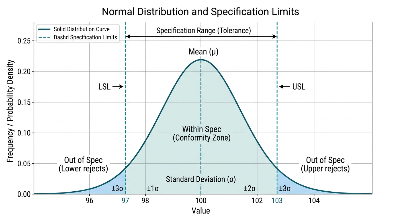
Figure 1 illustrates how a process with high variation, even if technically operating within tolerance limits, increases the risk of producing components near the boundaries. These borderline parts are highly prone to early-life failures, commonly classified as infant mortality in reliability engineering.
Figure 1: Normal distribution and specification limits
To quantify how well a process performs relative to its limits, reliability and quality managers use capability indices, primarily \(C_p\) and \(C_{pk}\). The \(C_p\) index measures the potential capability of a process, assuming it is perfectly centered between its specification limits:
$$C_p = \frac{\text{USL} - \text{LSL}}{6\sigma}$$
The \(C_{pk}\) index, however, accounts for any centering shift by measuring the distance from the process mean to the nearest specification limit:
$$C_{pk} = \min\left(\frac{\text{USL} - \mu}{3\sigma}, \frac{\mu - \text{LSL}}{3\sigma}\right)$$
Where \(\text{USL}\) is the Upper Specification Limit, \(\text{LSL}\) is the Lower Specification Limit, \(\mu\) is the process mean, and \(\sigma\) is the process standard deviation.
When a process is uncentered or highly variable, components are manufactured with asymmetric tolerances. This lack of precision directly degrades the operating life of the final product. Conversely, reducing variation ensures that assets run smoother, experience fewer micro-stops, and require less frequent maintenance interventions.
DMAIC in Action: Quantifying Process Variation
To systematically eliminate defects and variation, quality professionals use the DMAIC (Define, Measure, Analyze, Improve, Control) framework. Each phase of this methodology uses specific statistical tools to isolate root causes and establish permanent process control.
- Define: Identify the critical-to-quality (CTQ) characteristics of the product and map the boundaries of the manufacturing process.
- Measure: Collect baseline performance data, validate the measurement system using Gage Repeatability and Reproducibility (Gage R&R) studies to ensure measurement error is under 10% of total tolerance, and establish baseline process capability.
- Analyze: Use statistical testing (such as ANOVA and t-tests), regression analysis, and failure mode mapping to isolate the root causes of variation.
- Improve: Implement targeted solutions, optimize process parameters using Design of Experiments (DOE), and eliminate the root causes of defects.
- Control: Standardize the improved process and deploy statistical process control (SPC) to monitor performance over time.
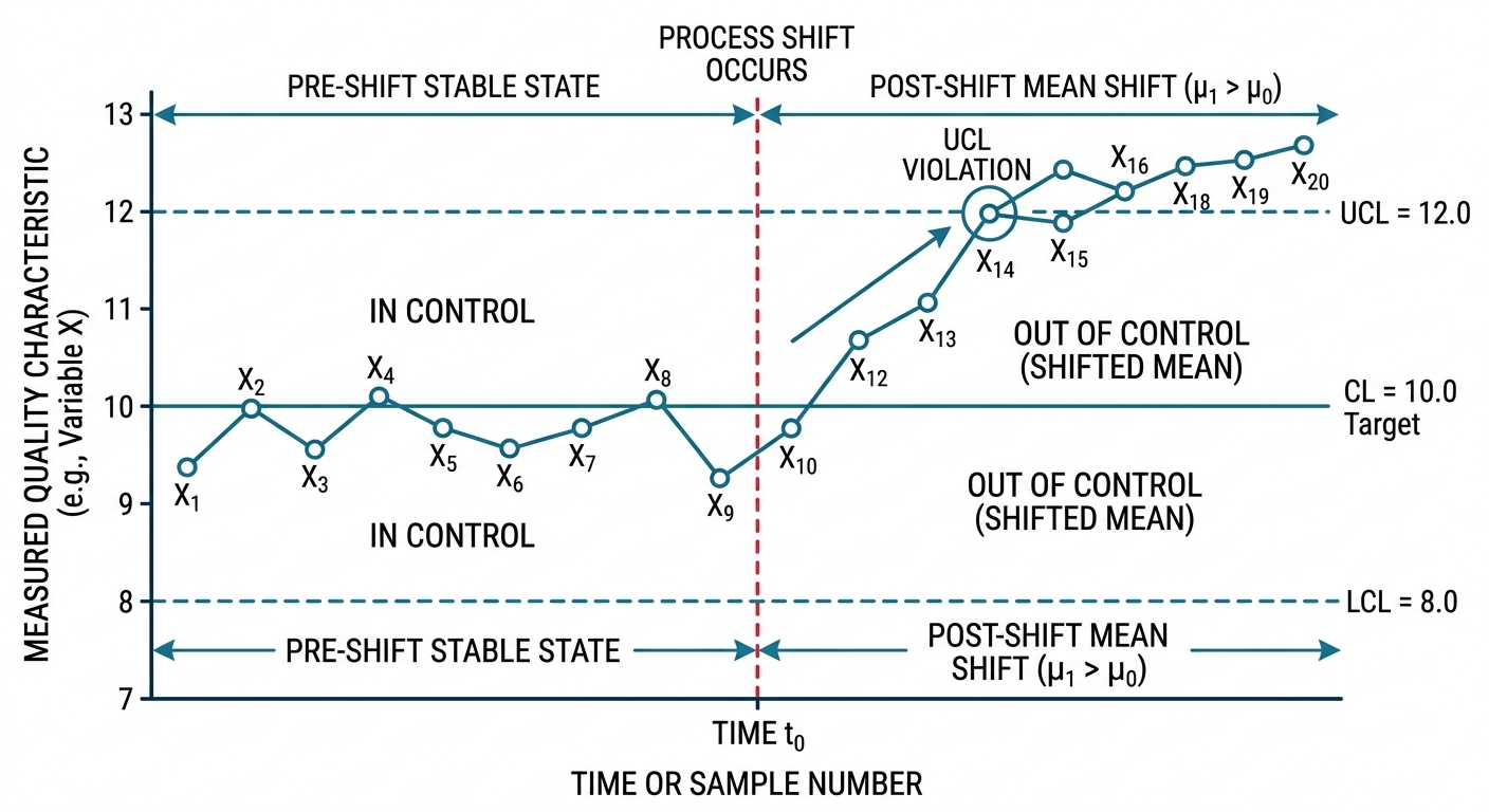
During the Control phase, engineers use the Control Chart Tool to detect non-random patterns, process shifts, or trends before they result in out-of-specification parts.
Figure 2: Control chart demonstrating process shift
To understand how process capability corresponds to overall defect rates and operational performance, consider the standard benchmarks outlined in the table below. Note that these metrics assume the industry-standard 1.5-sigma shift in the process mean over the long term.
| Process Capability (\(C_{pk}\)) | Process Sigma Level | Defects Per Million Opportunities (DPMO) | Operational Classification |
|---|---|---|---|
| < 1.00 | < 3.0\(\sigma\) | > 66,807 | Non-capable; high defect costs |
| 1.00 to 1.33 | 3.0\(\sigma\) to 4.0\(\sigma\) | 6,210 to 66,807 | Marginally capable; requires tight control |
| 1.33 to 1.67 | 4.0\(\sigma\) to 5.0\(\sigma\) | 233 to 6,210 | Capable; standard industrial benchmark |
| > 1.67 | > 5.0\(\sigma\) | < 233 | Highly capable; robust to process shifts |
| 2.00 | 6.0\(\sigma\) | 3.4 | World-class; near-zero defects |
A \(C_{pk}\) of 1.33 is the minimum acceptable benchmark for existing manufacturing processes, whereas new processes typically target a \(C_{pk}\) of 1.67 or higher to build in a safety margin against natural process drift.
Worked Example: Process Capability and DPMO Calculation
Consider a precision automotive manufacturing facility that produces drive shafts. The critical-to-quality dimension is the outer bearing journal diameter. The engineering specification for this diameter is set to:
- Nominal Target: 25.00 mm
- Upper Specification Limit (USL): 25.05 mm
- Lower Specification Limit (LSL): 24.95 mm
To evaluate the current process capability, a quality engineer collects a sample of 150 finished shafts over five consecutive production shifts. Statistical analysis of the sample yields:
- Sample Mean (\(\mu\)): 25.01 mm
- Sample Standard Deviation (\(\sigma\)): 0.012 mm
Because the sample mean (\(\mu = 25.01\) mm) is shifted slightly above the nominal target of 25.00 mm, we must calculate both \(C_p\) and \(C_{pk}\) to evaluate the true capability of the line.
Step 1: Calculate Potential Process Capability (\(C_p\))
The \(C_p\) index measures the ratio of the allowable tolerance spread to the actual process spread (defined as \(6\sigma\)).
$$C_p = \frac{\text{USL} - \text{LSL}}{6\sigma}$$
$$C_p = \frac{25.05 - 24.95}{6 \times 0.012}$$
$$C_p = \frac{0.10}{0.072} \approx 1.39$$
This indicates that if the process were perfectly centered at 25.00 mm, the process spread would easily fit within the specification limits.
Step 2: Calculate Actual Process Capability (\(C_{pk}\))
Because the process is shifted, we calculate the upper and lower capability indices (\(C_{pu}\) and \(C_{pl}\)) and take the minimum of the two.
$$C_{pu} = \frac{\text{USL} - \mu}{3\sigma} = \frac{25.05 - 25.01}{3 \times 0.012} = \frac{0.04}{0.036} \approx 1.11$$
$$C_{pl} = \frac{\mu - \text{LSL}}{3\sigma} = \frac{25.01 - 24.95}{3 \times 0.012} = \frac{0.06}{0.036} \approx 1.67$$
$$C_{pk} = \min(C_{pu}, C_{pl}) = \min(1.11, 1.67) = 1.11$$
The \(C_{pk}\) of 1.11 is significantly lower than the \(C_p\) of 1.39, indicating that process off-centering is consuming a substantial portion of the allowable tolerance.
Step 3: Calculate Defects Per Million Opportunities (DPMO)
To find the expected defect rate, we calculate the Z-scores for both specification limits and find the area under the standard normal curve outside these limits.
$$Z_{\text{upper}} = \frac{\text{USL} - \mu}{\sigma} = \frac{25.05 - 25.01}{0.012} = 3.33$$
$$Z_{\text{lower}} = \frac{\mu - \text{LSL}}{\sigma} = \frac{25.01 - 24.95}{0.012} = 5.00$$
Using standard normal distribution tables:
- The probability of a part exceeding the USL (\(Z > 3.33\)) is approximately \(0.000434\) (or 434 defects per million).
- The probability of a part falling below the LSL (\(Z < -5.00\)) is approximately \(0.000000287\) (essentially 0).
Adding these probabilities together yields a total defect rate of \(0.000434\), or 434 DPMO. To confirm these calculations or run a similar analysis on your own line, you can use the Process Capability Calculator and the DPMO Calculator.
Integrating Quality Tools with Reliability Engineering
A common pitfall in modern manufacturing is treating quality improvement and asset maintenance as separate disciplines. In practice, they are two sides of the same coin. When statistical quality methodologies are paired with reliability tools, engineers can target process variation that directly impacts asset wear.
For example, Failure Mode and Effects Analysis (FMEA) is a cornerstone of both disciplines. While a reliability engineer uses FMEA to analyze how a physical component might fail, a quality engineer uses Process FMEA (PFMEA) to evaluate how a process step might deviate. By combining these approaches, the facility can design out process variations that lead to mechanical failures.
Figure 3: Root cause variation analysis
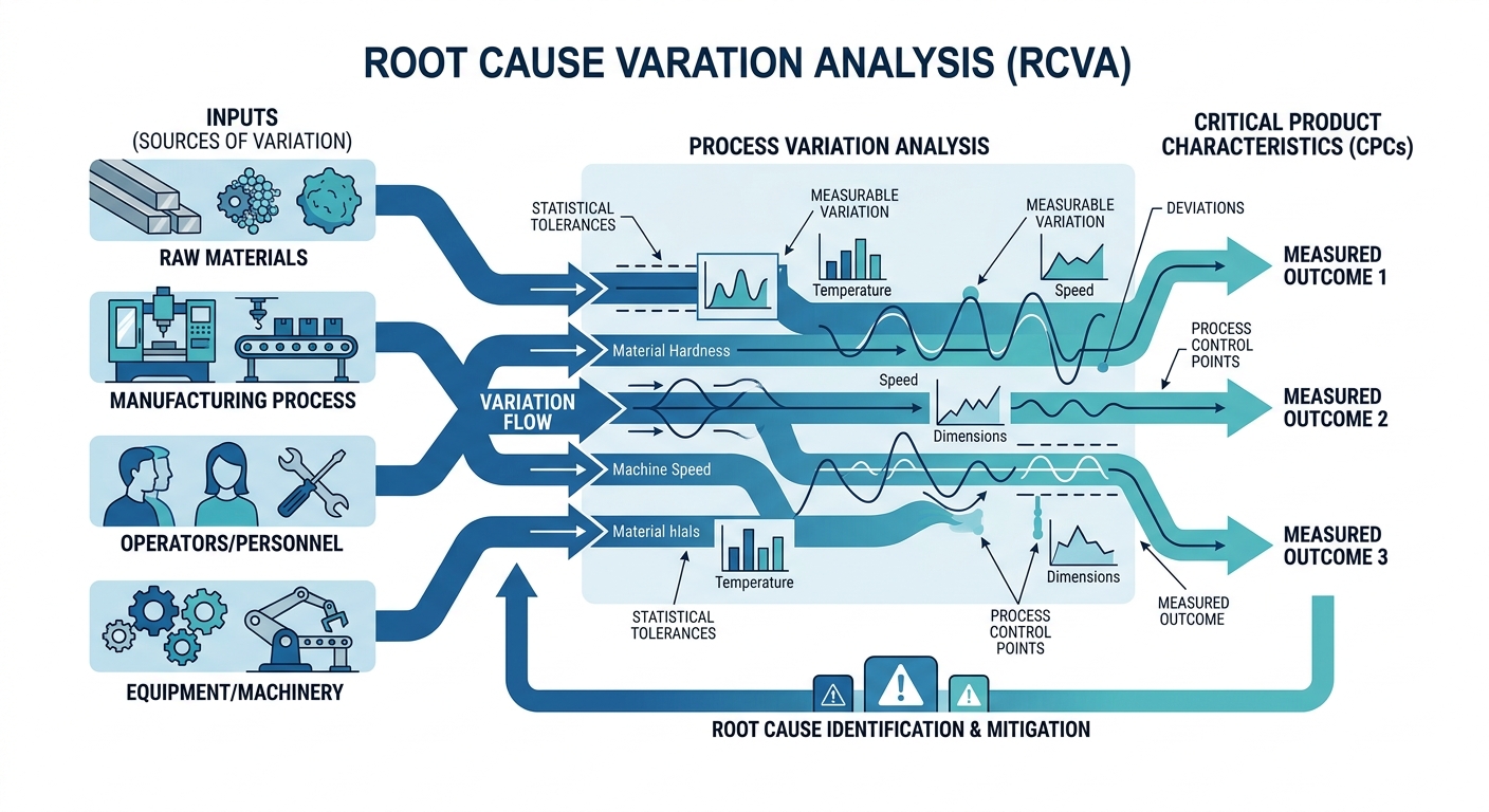
When process variation is reduced, machinery operates under steady-state conditions, reducing the thermal and mechanical stresses that cause premature component degradation. This synergy directly extends the life of tooling, bearings, and structural members, allowing maintenance teams to transition from reactive firefighting to a highly optimized, predictive maintenance model.
Conclusion
Reducing process variation is not merely an exercise in meeting quality specifications; it is a fundamental strategy for improving asset reliability and lowering operational costs. By measuring process capability, identifying centering errors, and applying systematic statistical controls, manufacturing organizations can eliminate the root causes of both product defects and equipment downtime. For interactive calculation tools, templates, and engineering guides designed to help you analyze process capability, calculate defect rates, and optimize asset uptime, visit the professional suite of tools available at ReliabilityCalc.com.