
Setting maintenance inspection intervals using arbitrary calendar schedules—such as fixed monthly visual checks or quarterly vibration routes—leads to two costly outcomes: undetected component failures or excessive technician labor spent inspecting healthy assets. Optimization requires anchoring task frequencies directly to physical degradation behavior. The P-F curve provides the mathematical framework for establishing defensible, risk-adjusted inspection schedules.
Mechanics of the P-F Curve and Degradation Windows
The P-F curve models defect progression from initial detection to functional failure. Point \(P\) (Potential Failure) represents the earliest point where a defect becomes detectable using a specific condition monitoring technique. Point \(F\) (Functional Failure) defines the threshold where the asset no longer meets its required operating performance.
Figure 1: P-F curve degradation profile
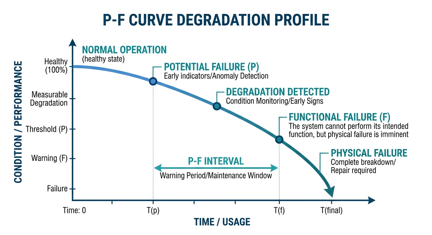
The elapsed time between Point \(P\) and Point \(F\) is the \(P\text{-}F\) interval (\(I_{PF}\)). This window defines the operational timeframe available to detect the anomaly, plan corrective work, procure spare parts, and execute repairs before an unplanned outage occurs.
The duration of \(I_{PF}\) is not an intrinsic equipment constant; it depends on the failure mode, operating severity, and diagnostic tool sensitivity. Advanced non-destructive testing (NDT) and high-frequency ultrasound detect subsurface fatigue months before damage manifests as heat or acoustic noise.
Mathematical Formulation of Optimal Inspection Frequencies
To guarantee detection before functional failure, inspection frequency must be shorter than the \(P\text{-}F\) interval. Classical reliability engineering applies the half-interval rule:
$$\Delta t \le \frac{I_{PF}}{2}$$
Setting \(\Delta t = \frac{I_{PF}}{2}\) ensures that at least one inspection cycle falls within the detection window between Point \(P\) and Point \(F\), even if a prior inspection occurred immediately before defect initiation crossed Point \(P\).
However, relying solely on this rule ignores key variables: missed detection probability (\(p_m\)), task execution costs (\(C_i\)), and failure consequence costs (\(C_d\)). To find the economic optimum, reliability engineers model total annual expected cost \(C_{total}(\Delta t)\) as a function of the inspection interval \(\Delta t\):
$$C_{total}(\Delta t) = C_{insp}(\Delta t) + C_{risk}(\Delta t)$$
$$C_{total}(\Delta t) = \left( \frac{365}{\Delta t} \cdot C_i \right) + \lambda \cdot P_{miss}(\Delta t) \cdot (C_d - C_p)$$
Where:
- \(C_i\) = Cost per single inspection route execution ($)
- \(\lambda\) = Expected failure rate per year (obtainable via the MTBF Calculator)
- \(p_m\) = Probability that a technician or tool misses an existing defect during an inspection (false negative rate)
- \(n = \lfloor \frac{I_{PF}}{\Delta t} \rfloor\) = Number of complete inspection cycles inside the \(P\text{-}F\) window
- \(P_{miss}(\Delta t) = (p_m)^n\) for \(\Delta t \le I_{PF}\), and \(P_{miss}(\Delta t) = 1 - (1 - p_m)\frac{I_{PF}}{\Delta t}\) for \(\Delta t > I_{PF}\)
- \(C_d\) = Total cost of an unmonitored failure (calculated via the Downtime Cost Calculator)
- \(C_p\) = Cost of planned corrective maintenance ($)
Figure 2: Cost tradeoff versus inspection frequency
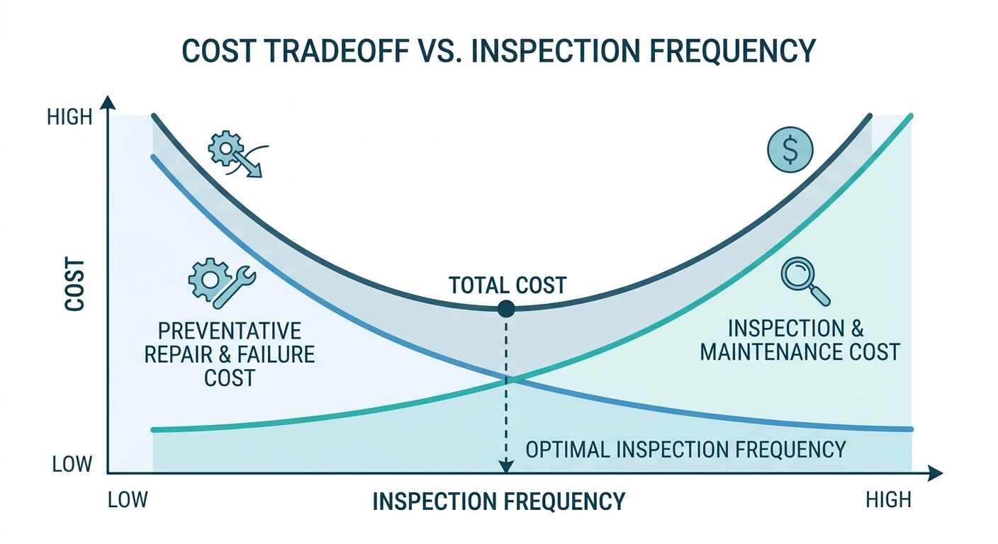
Evaluating \(C_{total}(\Delta t)\) across candidate intervals pinpoints the minimum-cost frequency that satisfies operational risk constraints.
Worked Example: Calculating Inspection Intervals for Rotating Assets
Consider a critical high-pressure boiler feed pump in continuous operation. We are designing an inspection schedule for rolling-element bearing fatigue.
Input Parameters
- Failure Mode: Bearing inner ring micro-spalling
- Detection Method: Vibration velocity spectrum analysis (\(10 \text{ Hz}\) to \(1 \text{ kHz}\))
- Determined \(P\text{-}F\) Interval (\(I_{PF}\)): \(60 \text{ days}\)
- Inspection Route Execution Cost (\(C_i\)): \(\$200 \text{ per route}\)
- Unplanned Failure Cost (\(C_d\)): \(\$85{,}000\) (includes secondary impeller damage, emergency overtime, and lost production)
- Planned Repair Cost (\(C_p\)): \(\$12{,}000\) (scheduled overhaul)
- Missed Detection Probability (\(p_m\)): \(0.10\) (\(10\%\))
- Historical Failure Rate (\(\lambda\)): \(0.15 \text{ failures/year}\) (\(\text{MTBF} = 6.67 \text{ years}\))
Step 1: Classical Baseline Interval
Applying the standard half-interval rule:
$$\Delta t_{baseline} = \frac{I_{PF}}{2} = \frac{60 \text{ days}}{2} = 30 \text{ days}$$
Evaluating every \(30 \text{ days}\) yields \(n = \lfloor \frac{60}{30} \rfloor = 2\) inspections within the \(P\text{-}F\) window.
Step 2: Risk Cost Calculation
With \(n = 2\) inspections inside \(I_{PF}\), the probability of missing the defect across both consecutive routes is:
$$P_{miss} = (p_m)^n = (0.10)^2 = 0.01 \text{ (1\%)}$$
The financial penalty differential between unplanned failure and planned repair is:
$$\Delta C = C_d - C_p = \$85{,}000 - \$12{,}000 = \$73{,}000$$
The expected annual risk cost \(C_{risk}\) for \(\Delta t = 30 \text{ days}\) is:
$$C_{risk}(30) = 0.15 \times 0.01 \times \$73{,}000 = \$109.50/\text{year}$$
Step 3: Annual Inspection Cost Calculation
For \(\Delta t = 30 \text{ days}\), the annual route frequency is \(\frac{365}{30} \approx 12.167\) inspections/year:
$$C_{insp}(30) = \left( \frac{365}{30} \right) \times \$200 = \$2{,}433.33/\text{year}$$
Total annual cost at \(30\text{-day}\) intervals:
$$C_{total}(30) = \$2{,}433.33 + \$109.50 = \$2{,}542.83/\text{year}$$
Step 4: Scenario Comparison (\(\Delta t = 15, 30, 60, \text{ and } 90 \text{ days}\))
Comparing candidate intervals:
For \(\Delta t = 15 \text{ days}\):
- \(n = \lfloor 60 / 15 \rfloor = 4\)
- \(P_{miss} = (0.10)^4 = 0.0001\)
- \(C_{risk}(15) = 0.15 \times 0.0001 \times \$73{,}000 = \$1.10/\text{year}\)
- \(C_{insp}(15) = \left( \frac{365}{15} \right) \times \$200 = \$4{,}866.67/\text{year}\)
- \(C_{total}(15) = \$4{,}866.67 + \$1.10 = \$4{,}867.77/\text{year}\)
For \(\Delta t = 60 \text{ days}\):
- \(n = \lfloor 60 / 60 \rfloor = 1\)
- \(P_{miss} = (0.10)^1 = 0.10\)
- \(C_{risk}(60) = 0.15 \times 0.10 \times \$73{,}000 = \$1{,}095.00/\text{year}\)
- \(C_{insp}(60) = \left( \frac{365}{60} \right) \times \$200 = \$1{,}216.67/\text{year}\)
- \(C_{total}(60) = \$1{,}216.67 + \$1{,}095.00 = \$2{,}311.67/\text{year}\)
For \(\Delta t = 90 \text{ days}\) (\(\Delta t > I_{PF}\)):
- \(P_{miss} = 1 - (1 - 0.10)\left(\frac{60}{90}\right) = 0.40\)
- \(C_{risk}(90) = 0.15 \times 0.40 \times \$73{,}000 = \$4{,}380.00/\text{year}\)
- \(C_{insp}(90) = \left( \frac{365}{90} \right) \times \$200 = \$811.11/\text{year}\)
- \(C_{total}(90) = \$811.11 + \$4{,}380.00 = \$5{,}191.11/\text{year}\)
Although \(\Delta t = 60 \text{ days}\) shows a slightly lower total annual cost than \(30 \text{ days}\) (\(\$2{,}311.67\) vs. \(\$2{,}542.83\)), it leaves only \(n = 1\) inspection inside \(I_{PF}\). If that single check misses the defect due to noise or human error, an unmonitored failure occurs. Selecting \(\Delta t = 30 \text{ days}\) is the defensible engineering choice, providing a \(99\%\) cumulative detection probability for a minimal \(\$231.16\)/year premium.
Comparing Condition Monitoring Modalities and Detection Horizons
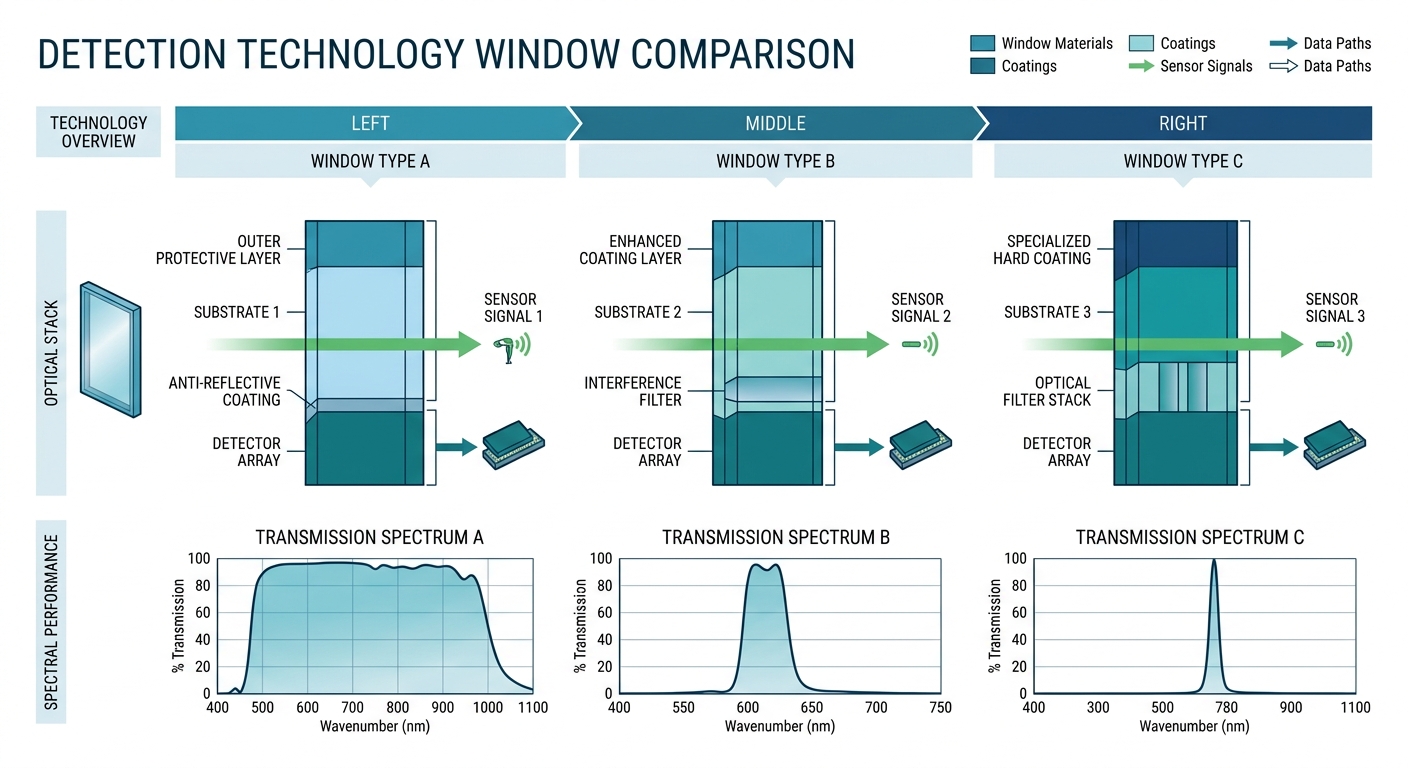
Selecting diagnostic technology dictates where Point \(P\) falls on the degradation curve. Higher-sensitivity modalities shift Point \(P\) earlier, extending \(I_{PF}\) and enabling longer, lower-cost inspection intervals.
Figure 3: Detection technology window comparison
| Monitoring Modality | Typical \(P\text{-}F\) Window (\(I_{PF}\)) | Relative Point \(P\) Position | Primary Failure Modes Detected | Inspection Cost per Asset |
|---|---|---|---|---|
| High-Frequency Ultrasound | \(90 \text{ to } 180 \text{ days}\) | Very Early | Subsurface friction, early bearing micro-spalling | Low |
| Oil Analysis / Spectrometry | \(60 \text{ to } 120 \text{ days}\) | Early | Gear/bearing wear particles, oil contamination | Medium |
| Vibration Velocity Analysis | \(30 \text{ to } 60 \text{ days}\) | Moderate | Unbalance, misalignment, looseness, structural resonance | Medium |
| Infrared Thermography | \(10 \text{ to } 30 \text{ days}\) | Late | Electrical connection heating, coupling wear, lubrication breakdown | Low |
| Audible / Tactile Inspection | \(1 \text{ to } 5 \text{ days}\) | Very Late | Severe mechanical damage already in progress | Very Low |
The practical implication is that sensing technology and inspection interval must be selected together. Upgrading from a \(60\text{-day}\) vibration window to ultrasound with \(I_{PF} = 120 \text{ days}\) doubles the feasible \(\Delta t\) at the same \(n = 2\) detection redundancy, roughly halving annual route cost without sacrificing detection probability.
Conclusion
The P-F curve reframes inspection scheduling as a quantitative trade-off rather than a calendar habit. Estimate \(I_{PF}\) for the dominant failure mode, require at least \(n = 2\) detection opportunities inside the window, and confirm the choice economically by comparing \(C_{total}(\Delta t)\) across candidate intervals — in the worked example above, the \(30\text{-day}\) route earns its \(\$231.16\)/year premium by lifting cumulative detection probability from \(90\%\) to \(99\%\). Revisit the calculation whenever failure rates, repair costs, or monitoring technology change. For the supporting inputs, the MTBF Calculator and the other reliability tools at ReliabilityCalc.com make each recalculation a five-minute exercise.