
When a high-pressure hydraulic valve spool exhibits intermittent binding during field operation despite passing final dimensional inspection, the failure is rarely an isolated machining anomaly. In automated production, such defects usually stem from unmanaged process dispersion and subtle mean shifts that accumulate across extended manufacturing runs. Post-process inspection merely separates conforming parts from scrap; it cannot quantify whether a process possesses the statistical margin to meet engineering specifications reliably.
To evaluate manufacturing performance systematically, quality and reliability engineers rely on process capability (\(C_p, C_{pk}\)) and process performance (\(P_p, P_{pk}\)) indices. These metrics quantify the alignment between the inherent statistical variability of a process and its specification limits.
Short-Term Capability vs. Long-Term Performance
Evaluating a manufacturing process requires distinguishing between short-term potential capability and long-term realized performance. This distinction depends on sampling methodology and how standard deviation is estimated.
Short-term capability metrics (\(C_p, C_{pk}\)) quantify process behavior under controlled conditions over brief operational windows. During these intervals, common-cause variation—such as minor mechanical vibration or baseline hydraulic pressure fluctuations—dominates the data. Special-cause variation (e.g., raw material lot shifts, operator adjustments, ambient temperature swings, and tool wear) is minimized. Short-term data is collected using rational subgrouping, where samples are gathered close together in time.
Conversely, long-term performance metrics (\(P_p, P_{pk}\)) evaluate output across extended production runs (days, weeks, or months). This longitudinal sampling captures both common-cause and special-cause variation. While short-term metrics define what a process can achieve under ideal, stable conditions, long-term metrics quantify actual quality delivered to the customer.
Figure 1: Short term versus long term variation spread
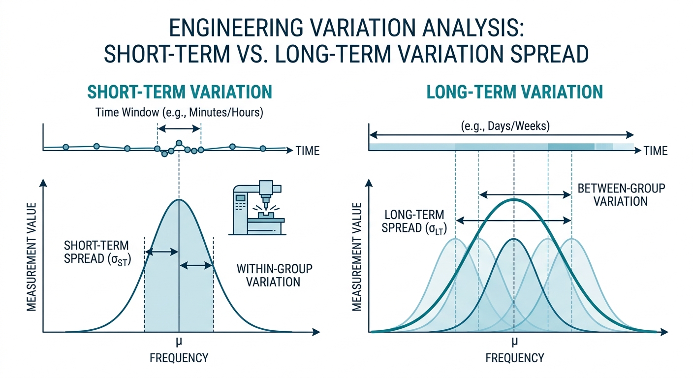
A process can exhibit high short-term capability while delivering poor long-term performance. This divergence occurs when unmonitored environmental shifts or mechanical wear drift the process mean away from nominal design targets over time.
Mathematical Formulations and Estimators
Calculating process capability and performance requires precise mathematical definitions of centering and dispersion relative to the Upper Specification Limit (\(\text{USL}\)) and Lower Specification Limit (\(\text{LSL}\)). The total allowable specification width is \(\text{USL} - \text{LSL}\).
Capability Indices (\(C_p\) and \(C_{pk}\))
The potential capability index, \(C_p\), measures the ratio of allowable engineering tolerance to the inherent short-term process spread (\(6\sigma_{\text{within}}\)). It assumes the process mean is perfectly centered between specification limits:
$$C_p = \frac{\text{USL} - \text{LSL}}{6\sigma_{\text{within}}}$$
Because \(C_p\) ignores process centering, it represents the upper bound of capability achievable if the process mean aligns perfectly with the nominal midpoint.
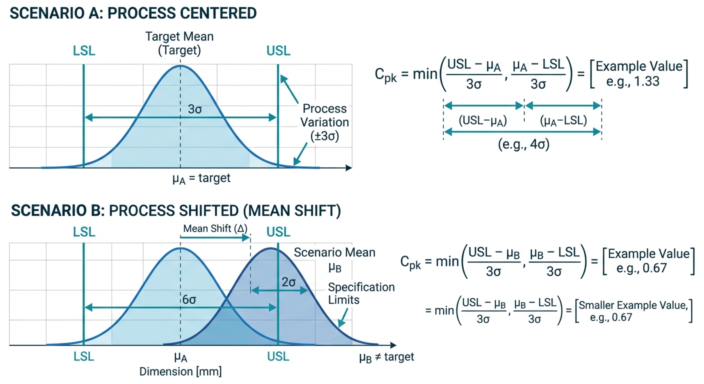
To account for off-center operation, the actual capability index, \(C_{pk}\), evaluates the distance from the process mean (\(\mu\)) to the nearest specification limit, normalized by three standard deviations (\(3\sigma_{\text{within}}\)):
$$C_{pk} = \min\left( \frac{\text{USL} - \mu}{3\sigma_{\text{within}}}, \frac{\mu - \text{LSL}}{3\sigma_{\text{within}}} \right)$$
In short-term evaluations, \(\sigma_{\text{within}}\) is estimated from subgroup data using unbiasing constants. When using average subgroup ranges (\(\bar{R}\)), the estimator is:
$$\sigma_{\text{within}} = \frac{\bar{R}}{d_2}$$
where \(\bar{R}\) is the average range across \(k\) subgroups and \(d_2\) is an unbiasing constant based on subgroup sample size \(n\). You can compute control limits and short-term dispersion metrics automatically using the Control Chart Tool.
Figure 2: Effect of mean centering shift on Cpk
Performance Indices (\(P_p\) and \(P_{pk}\))
Performance indices use identical structural equations but replace \(\sigma_{\text{within}}\) with the overall sample standard deviation (\(s_{\text{overall}}\)) computed across the entire combined dataset:
$$P_p = \frac{\text{USL} - \text{LSL}}{6s_{\text{overall}}}$$
$$P_{pk} = \min\left( \frac{\text{USL} - \bar{X}}{3s_{\text{overall}}}, \frac{\bar{X} - \text{LSL}}{3s_{\text{overall}}} \right)$$
The overall sample standard deviation \(s_{\text{overall}}\) is calculated via standard sample variance:
$$s_{\text{overall}} = \sqrt{\frac{\sum_{i=1}^{N} (X_i - \bar{X})^2}{N - 1}}$$
Because \(s_{\text{overall}}\) reflects shift-to-shift drift, operator variability, thermal expansion, and tool wear, \(s_{\text{overall}} \ge \sigma_{\text{within}}\) for real-world operations, making \(P_{pk} \le C_{pk}\) in non-ideal processes.
Worked Engineering Example: Machining Hydraulic Valve Spools
Consider a CNC turning operation producing outer spool diameters for high-pressure hydraulic control valves.
Process Parameters
- Lower Specification Limit (\(\text{LSL}\)): \(24.950\text{ mm}\)
- Upper Specification Limit (\(\text{USL}\)): \(25.050\text{ mm}\)
- Tolerance Width (\(\text{USL} - \text{LSL}\)): \(0.100\text{ mm}\)
- Sampling Plan: \(k = 20\) subgroups of size \(n = 5\) (\(N = 100\) total measurements)
Data Summary Statistics
- Grand Mean (\(\bar{X}\)): \(25.012\text{ mm}\)
- Average Subgroup Range (\(\bar{R}\)): \(0.018\text{ mm}\)
- Unbiasing Constant (\(d_2\) for \(n = 5\)): \(2.326\)
- Overall Standard Deviation (\(s_{\text{overall}}\)): \(0.009450\text{ mm}\)
Step-by-Step Calculations
Step 1: Estimate short-term within-subgroup standard deviation (\(\sigma_{\text{within}}\)):
$$\sigma_{\text{within}} = \frac{\bar{R}}{d_2} = \frac{0.018}{2.326} \approx 0.007739\text{ mm}$$
Step 2: Calculate potential capability (\(C_p\)):
$$C_p = \frac{25.050 - 24.950}{6 \times 0.007739} = \frac{0.100}{0.046434} \approx 2.154$$
Step 3: Calculate actual short-term capability (\(C_{pk}\)):
$$C_{pk, \text{upper}} = \frac{25.050 - 25.012}{3 \times 0.007739} = \frac{0.038}{0.023217} \approx 1.637$$
$$C_{pk, \text{lower}} = \frac{25.012 - 24.950}{3 \times 0.007739} = \frac{0.062}{0.023217} \approx 2.670$$
$$C_{pk} = \min(1.637, 2.670) = 1.637$$
Step 4: Calculate overall potential performance (\(P_p\)):
$$P_p = \frac{25.050 - 24.950}{6 \times 0.009450} = \frac{0.100}{0.056700} \approx 1.764$$
Step 5: Calculate overall actual performance (\(P_{pk}\)):
$$P_{pk, \text{upper}} = \frac{25.050 - 25.012}{3 \times 0.009450} = \frac{0.038}{0.028350} \approx 1.340$$
$$P_{pk, \text{lower}} = \frac{25.012 - 24.950}{3 \times 0.009450} = \frac{0.062}{0.028350} \approx 2.187$$
$$P_{pk} = \min(1.340, 2.187) = 1.340$$
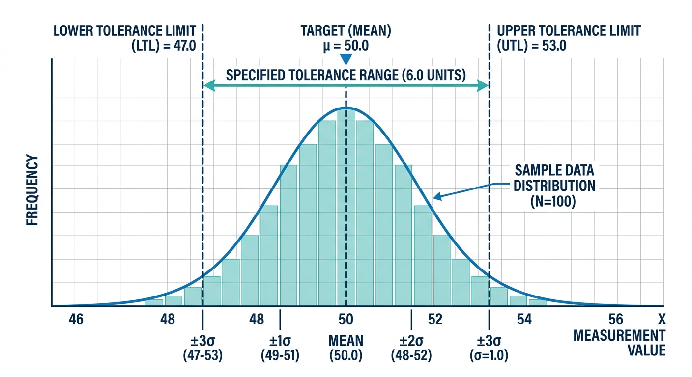
Figure 3: Sample data distribution against tolerance limits
Technical Interpretation
The process yields \(C_p = 2.154\), proving that instantaneous equipment precision easily fits within the \(0.100\text{ mm}\) tolerance band. However, \(C_{pk}\) drops to \(1.637\) because the mean (\(25.012\text{ mm}\)) has shifted \(+0.012\text{ mm}\) toward the upper limit.
Furthermore, long-term performance degrades to \(P_{pk} = 1.340\). The gap between \(C_{pk} (1.637)\) and \(P_{pk} (1.340)\) reveals significant long-term variation sources, such as thermal expansion of the lathe spindle and cutting tool wear. Engineers can verify these calculations using the Process Capability Calculator and translate these indices into projected defect rates using a DPMO Calculator.
Decision Framework and Benchmark Criteria
Industrial engineering standards establish minimum capability targets based on process criticality and risk severity.
| Index Target (\(C_{pk} / P_{pk}\)) | Sigma Equivalent | Expected Defect Rate (PPM) | Process Status & Required Action |
|---|---|---|---|
| \(< 1.00\) | \(< 3.0\sigma\) | \(> 2{,}700\) | Non-Conforming: Excessive scrap/rework. Halt production or mandate \(100\%\) sorting inspection. |
| \(1.00 - 1.33\) | \(3.0\sigma - 4.0\sigma\) | \(2{,}700 - 64\) | Marginal: Meets basic tolerances but lacks safety margin. Mandate active SPC controls. |
| \(1.33 - 1.67\) | \(4.0\sigma - 5.0\sigma\) | \(64 - 0.57\) | Capable: Standard requirement for critical industrial and automotive components. |
| \(> 1.67\) | \(> 5.0\sigma\) | \(< 0.57\) | Superior: Recommended for aerospace, medical device, and life-critical applications. |
Evaluating the ratio of long-term performance to short-term capability provides a diagnostic metric for process stability:
$$\text{Capability Ratio} = \frac{P_{pk}}{C_{pk}}$$
- Ratio \(\ge 0.90\): Highly controlled process with negligible special-cause drift over time.
- Ratio \(< 0.75\): Severe process instability. Systemic factors—such as shift changeovers, thermal drift, or raw material batch variation—are degrading long-term yields.
Poor capability directly compromises operational equipment efficiency. Defective components cause line stoppages, re-work loops, and premature field failures. Integrating capability data into an OEE Calculator ensures quality losses are fully represented in plant performance metrics.
Root Cause Diagnostics for Low Capability Metrics
When capability falls below target thresholds, engineers can isolate the root cause by evaluating the relationship between metrics:
High \(C_p\), Low \(C_{pk}\) (\(C_p \gg C_{pk}\)):
- Diagnosis: Process dispersion is narrow, but the mean is off-center.
- Corrective Action: Adjust machine tool offsets, recalibrate sensor baselines, or re-center control limits. This is typically a low-cost, quick-fix correction.
Low \(C_p\), Low \(C_{pk}\) (\(C_p \approx C_{pk} < 1.33\)):
- Diagnosis: Intrinsic short-term variation is too large relative to specification limits.
- Corrective Action: Perform mechanical maintenance, rebuild machine spindles, upgrade tool holding fixtures, or loosen non-critical design tolerances. Re-centering alone will not solve the issue.
High \(C_{pk}\), Low \(P_{pk}\) (\(P_{pk} / C_{pk} < 0.75\)):
- Diagnosis: Short-term precision is acceptable, but extended operations suffer from environmental, setup, or tool-wear drift.
- Corrective Action: Implement automated tool-wear offset compensation, standardize operator setup procedures, add active ambient temperature control, or tighten incoming raw material acceptance limits.
Systematic calculation of \(C_p\), \(C_{pk}\), \(P_p\), and \(P_{pk}\) moves quality control from reactive defect detection to predictive process prevention. To evaluate your manufacturing data, model tolerance limits, and automate statistical quality calculations, access the suite of technical tools available at ReliabilityCalc.com.