
When a high-speed bottling line rated at 300 units per minute (UPM) consistently averages an output of only 180 UPM over a 12-hour shift, plant management often defaults to blaming capital equipment limitations. However, a systematic decomposition of the asset's performance usually reveals a combination of micro-stops, prolonged changeovers, and minor quality deviations.
Maximizing the productivity of physical assets requires a rigorous approach to identifying, measuring, and eliminating these hidden losses. By systematically analyzing the core components of equipment utilization, reliability teams can transition from reactive troubleshooting to structured, data-driven optimization.
Deconstructing the Loss Landscape
To systematically improve asset utilization, you must first isolate losses into three distinct, measurable categories: Availability, Performance, and Quality. These three metrics serve as the foundation of Overall Equipment Effectiveness (OEE). While many facilities track these metrics at a high level, true optimization requires mapping specific floor-level events to the "Six Big Losses" defined within manufacturing reliability frameworks.
[Planned Production Time]
       │
       ├──► [Availability Losses] (Breakdowns, Setups/Adjustments)
       │           │
       │           └──► [Operating Time]
       │                      │
       │                      ├──► [Performance Losses] (Minor Stops, Reduced Speed)
       │                      │           │
       │                      │           └──► [Net Operating Time]
       │                      │                      │
       │                      │                      ├──► [Quality Losses] (Rejects, Startup Yield)
       │                      │                      │           │
       │                      │                      │           └──► [Valuable Operating Time]
Figure 1: Decomposition of manufacturing losses from planned time to valuable output
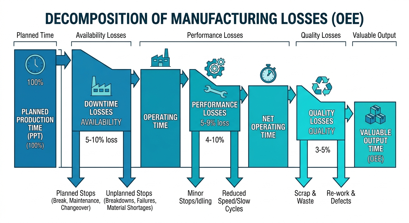
To bridge the gap between high-level metrics and floor-level execution, reliability engineers must map these three categories directly to the Six Big Losses:
- Unplanned Stops (Availability Loss): Sudden mechanical or electrical failures, critical component wear, or utility outages.
- Setup and Adjustments (Availability Loss): Tooling changeovers, warm-up periods, material replenishment, and calibration cycles.
- Small Stops (Performance Loss): Micro-stoppages (typically under two minutes) caused by sensor misalignments, feed jams, or minor clearance issues that do not require maintenance intervention.
- Slow Cycles (Performance Loss): Equipment running below its nameplate design speed due to mechanical wear, improper lubrication, or operator-imposed speed overrides.
- Production Rejects (Quality Loss): Scrap, rework, and out-of-specification parts generated during steady-state production.
- Startup Rejects (Quality Loss): Yield losses and scrap generated during warm-up, changeover stabilization, or process adjustments.
To establish an accurate baseline before implementing changes, engineers can utilize the OEE Calculator to quantify these losses. Tracking these components individually prevents a high score in one area (such as Quality) from masking severe deficiencies in another (such as Availability).
Targeted Engineering Techniques for Availability Losses
Availability losses are typically the most visible disruptions on the production floor. Minimizing them requires a dual-pronged approach: reducing the duration of planned stoppages and decreasing the frequency of unplanned failures.
Single-Minute Exchange of Die (SMED)
For planned stoppages like product changeovers, the SMED methodology is the primary engineering standard. The technique categorizes setup activities into internal elements (actions that must be performed while the machine is stopped) and external elements (actions that can be performed while the machine is running).
Implementing SMED involves a structured four-step process:
- Identify: Document and video-record the current changeover process to isolate every step, tool, and movement.
- Separate: Classify each step as strictly internal or external. For example, retrieving a new mold is external, while bolting it to the press is internal.
- Convert: Redesign tasks to move them from internal to external. This includes pre-heating molds, pre-staging raw materials, and pre-calibrating tooling before the machine stops.
- Streamline: Optimize the remaining internal tasks. Replace threaded fasteners with quick-release pneumatic clamps, slide-in guides, or standardized spacer blocks to eliminate manual adjustments.
Reliability-Centered Maintenance (RCM)
Unplanned breakdowns require a transition from reactive run-to-failure practices to proactive maintenance strategies. Utilizing a structured FMEA Tool allows reliability engineers to identify failure modes before they manifest as physical stoppages.
[Identify Asset] ──► [Define Functions] ──► [Identify Failure Modes] ──► [Evaluate Criticality] ──► [Apply PM/PdM Tasks]
Figure 2: Reliability-Centered Maintenance workflow for critical assets
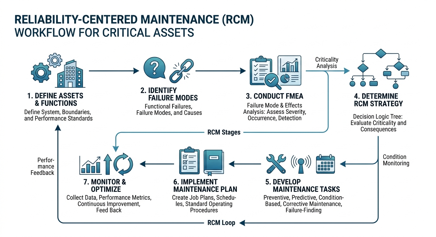
By implementing predictive maintenance (PdM) technologies such as vibration analysis, ultrasonic emission monitoring, and oil spectrography, maintenance teams can identify degradation curves (P-F intervals) early. This allows maintenance to be scheduled during planned windows, preserving availability.
When failures do occur, tracking metrics like Mean Time To Repair with the MTTR Calculator helps identify tooling bottlenecks, training gaps, or spare parts availability issues that extend downtime. Conversely, monitoring the Mean Time Between Failures using the MTBF Calculator provides direct visibility into the structural reliability of the asset.
Worked Mathematical Example: Diagnosing and Calculating OEE
To illustrate how these losses interact, consider a manufacturing line operating a single 8-hour shift. The following calculations demonstrate how to isolate losses and calculate the overall performance metric.
Step 1: Define the Input Parameters
- Total Shift Length: 8 hours (480 minutes)
- Planned Downtime: 30 minutes (scheduled preventative maintenance and operator breaks)
- Unplanned Downtime: 45 minutes (sensor failure and subsequent troubleshooting)
- Setup & Changeover Time: 25 minutes
- Ideal Cycle Time: 0.40 seconds per unit (or 150 units per minute / 9,000 units per hour)
- Total Output Produced: 48,000 units
- Defective Units: 1,200 units (rejected by vision inspection system)
Step 2: Calculate Availability (\(A\))
First, determine the Planned Production Time:
$$\text{Planned Production Time} = \text{Shift Length} - \text{Planned Downtime}$$
$$\text{Planned Production Time} = 480\text{ min} - 30\text{ min} = 450\text{ minutes}$$
Next, determine the actual Run Time:
$$\text{Run Time} = \text{Planned Production Time} - (\text{Unplanned Downtime} + \text{Setup Time})$$
$$\text{Run Time} = 450\text{ min} - (45\text{ min} + 25\text{ min}) = 380\text{ minutes}$$
Now, compute Availability:
$$A = \frac{\text{Run Time}}{\text{Planned Production Time}} = \frac{380\text{ min}}{450\text{ min}} \approx 0.8444\text{ (84.44\%)}$$
Step 3: Calculate Performance (\(P\))
Performance measures how close the machine ran to its maximum designed speed during the active Run Time:
$$P = \frac{\text{Ideal Cycle Time} \times \text{Total Output}}{\text{Run Time}}$$
Convert the Ideal Cycle Time to minutes per unit:
$$\text{Ideal Cycle Time} = \frac{0.40\text{ seconds}}{60\text{ seconds/minute}} \approx 0.006667\text{ minutes per unit}$$
Calculate Performance:
$$P = \frac{0.006667\text{ min/unit} \times 48,000\text{ units}}{380\text{ minutes}} = \frac{320\text{ minutes of work}}{380\text{ minutes of running}} \approx 0.8421\text{ (84.21\%)}$$
This indicates that minor stops and speed reductions accounted for 60 minutes of lost operating time during the run.
Step 4: Calculate Quality (\(Q\))
Quality measures the ratio of good parts produced to total parts started:
$$\text{Good Units} = \text{Total Output} - \text{Defective Units}$$
$$\text{Good Units} = 48,000 - 1,200 = 46,800\text{ units}$$
$$Q = \frac{\text{Good Units}}{\text{Total Output}} = \frac{46,800}{48,000} = 0.9750\text{ (97.50\%)}$$
Step 5: Calculate OEE
Multiply the three components to find the final metric:
$$\text{OEE} = A \times P \times Q$$
$$\text{OEE} = 0.8444 \times 0.8421 \times 0.9750 \approx 0.6933\text{ (69.33\%)}$$
This calculation reveals that while no individual metric fell below 84%, the compound effect of these losses resulted in an overall equipment effectiveness of just 69.33%.
Performance and Quality Optimization Strategies
Once Availability is stabilized, reliability engineers must address Performance and Quality losses. Performance losses are frequently driven by micro-stops (stoppages lasting less than two minutes) that operators resolve quickly without logging them in the CMMS. Quality losses, on the other hand, are driven by process instability and tool wear.
| Loss Category | Primary Failure Mode | Engineering Strategy | Analytical Tool / Metric |
|---|---|---|---|
| Availability | Component wear, long setups | SMED, Predictive Maintenance (PdM) | MTBF, MTTR |
| Performance | Misalignments, micro-stops | Chronocycle analysis, PLC log analysis | Speed Loss Index |
| Quality | Process drift, tooling degradation | Statistical Process Control (SPC), Poka-Yoke | \(C_p\), \(C_{pk}\) indices |
To resolve minor stops, engineers should perform high-speed video analysis or audit PLC event logs to identify recurring sensor faults or feed-chute jams.
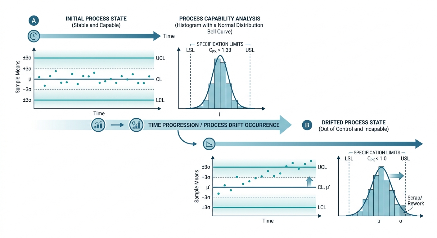
For quality issues, relying on end-of-line inspection is insufficient because it only identifies defects after the energy and raw materials have already been consumed. Instead, process engineers must apply Statistical Process Control (SPC) to monitor critical-to-quality variables in real time.
By analyzing process variation using the Process Capability Calculator, quality managers can determine whether a machine is statistically capable of holding its tolerances. If the process capability index (\(C_{pk}\)) is below 1.33, the process is highly susceptible to generating defects as the tooling wears or environmental conditions drift.
Lower Spec Limit (LSL)             Target             Upper Spec Limit (USL)
         │                           │                           │
         │         ┌───┐             │             ┌───┐         │
         │      ┌──┘   └──┐          │          ┌──┘   └──┐      │
         ├──────┘         └──────────┼──────────┘         └──────┤
         │   Process Out of Control  │      Process In Control   │
Figure 3: Statistical Process Control limits indicating process capability drift
Implementing automated Poka-Yoke (mistake-proofing) mechanisms—such as physical guide rails that prevent misaligned parts from entering a press, or photoelectric sensors that verify part presence before a cycle begins—effectively eliminates human error as a source of quality loss.
Conclusion
Optimizing equipment effectiveness is not a one-time project; it is an iterative engineering discipline. By decomposing asset performance into Availability, Performance, and Quality, reliability professionals can identify the precise root causes of lost manufacturing capacity. Whether the solution involves executing SMED workshops to reduce changeover times, deploying predictive maintenance strategies to extend the interval between breakdowns, or utilizing SPC to prevent quality drift, decisions must always be guided by rigorous, quantitative metrics.
For engineers and quality managers looking to streamline these analytical steps, a suite of dedicated tools is available at ReliabilityCalc.com. These resources, including specialized calculators for reliability, availability, and process capability, help simplify complex data analysis on the production floor.