
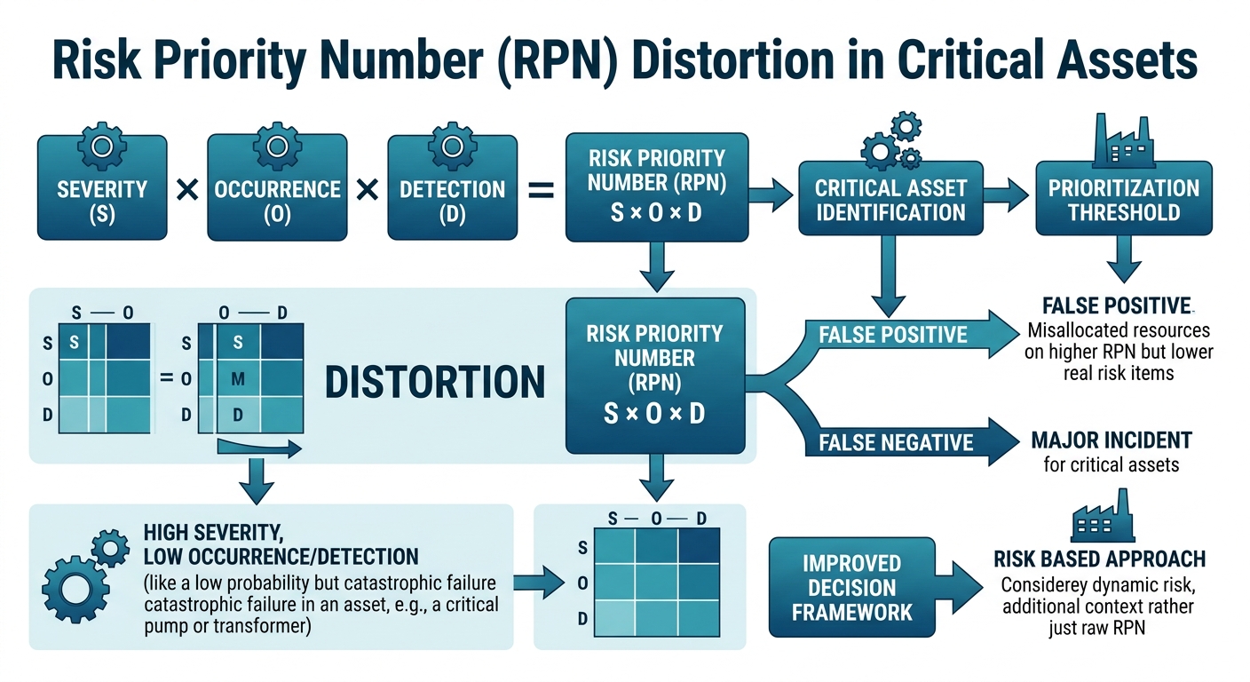
A plant manager reviewing a hydraulic press line failure mode and effects analysis (FMEA) notices two distinct failure modes assigned an identical composite Risk Priority Number (RPN) of 120:
- O-Ring Degradation: Gradual elastomeric seal breakdown causing a 0.5-liter/hour hydraulic fluid leak (\(S=3, O=5, D=8 \implies \text{RPN} = 120\)).
- Main Cylinder Tie-Rod Shear: Fatigue fracture dropping a 12-ton ram without warning (\(S=10, O=2, D=6 \implies \text{RPN} = 120\)).
Under a typical plant policy requiring engineering action only for scores exceeding 150, neither failure mode triggers capital allocation. Yet the tie-rod fracture introduces catastrophic safety hazards and severe downtime risks, while the seal weep is a routine maintenance task.
Standard multiplicative scoring frequently masks critical failure modes due to ordinal scale distortions. Establishing a resilient risk management framework requires moving beyond simplistic mathematical products toward structured, empirically grounded prioritization methods.
Figure 1: Risk priority number distortion in critical assets
The Mathematical Limitations of Traditional RPN Metrics
The traditional Risk Priority Number evaluates risk using three discrete ordinal rankings: Severity (\(S\)), Occurrence (\(O\)), and Detection (\(D\)).
$$\text{RPN} = S \cdot O \cdot D$$
Although straightforward to compute, multiplying these ordinal ratings introduces three severe mathematical flaws in reliability engineering:
- Ordinal Scale Multiplication: Severity, Occurrence, and Detection ratings are non-interval, non-ratio ordinal ranks (typically 1 to 10). Arithmetically multiplying ordinal values is mathematically invalid because the distance between scores of 2 and 3 does not equal the distance between 8 and 9. Ordinal numbers denote sequence, not absolute magnitude.
- Scale Gaps and Domain Compression: A 1–10 rating scale across three factors yields \(10^3 = 1{,}000\) possible combinations, but produces only 120 unique mathematical products. Over 88% of the 1–1000 domain contains empty values, creating dense clusters at low RPN values and extreme gaps among higher values.
- Mathematical Equivalence of Non-Equivalent Risks: High-severity events are mathematically identical to high-frequency, low-impact events under basic multiplication. For example, \(S=10, O=1, D=2 \implies \text{RPN}=20\) yields the exact same product as \(S=2, O=5, D=2 \implies \text{RPN}=20\). Treating catastrophic single-point failures identically to minor recurring annoyances compromises safety, regulatory compliance, and asset protection.
To overcome these structural flaws, engineering teams must anchor evaluation scales to quantifiable plant metrics and implement structured decision logic. Using a dedicated FMEA Tool allows teams to maintain clear line-of-sight between ordinal rankings and real-world operational risk.
Calibrating Severity, Occurrence, and Detection Scales
An effective risk evaluation framework replaces subjective engineering estimates with objective definitions grounded in physical data, downtime costs, and time-to-detect intervals.
Figure 2: Calibration matrix mapping quantitative metrics to ordinal ratings
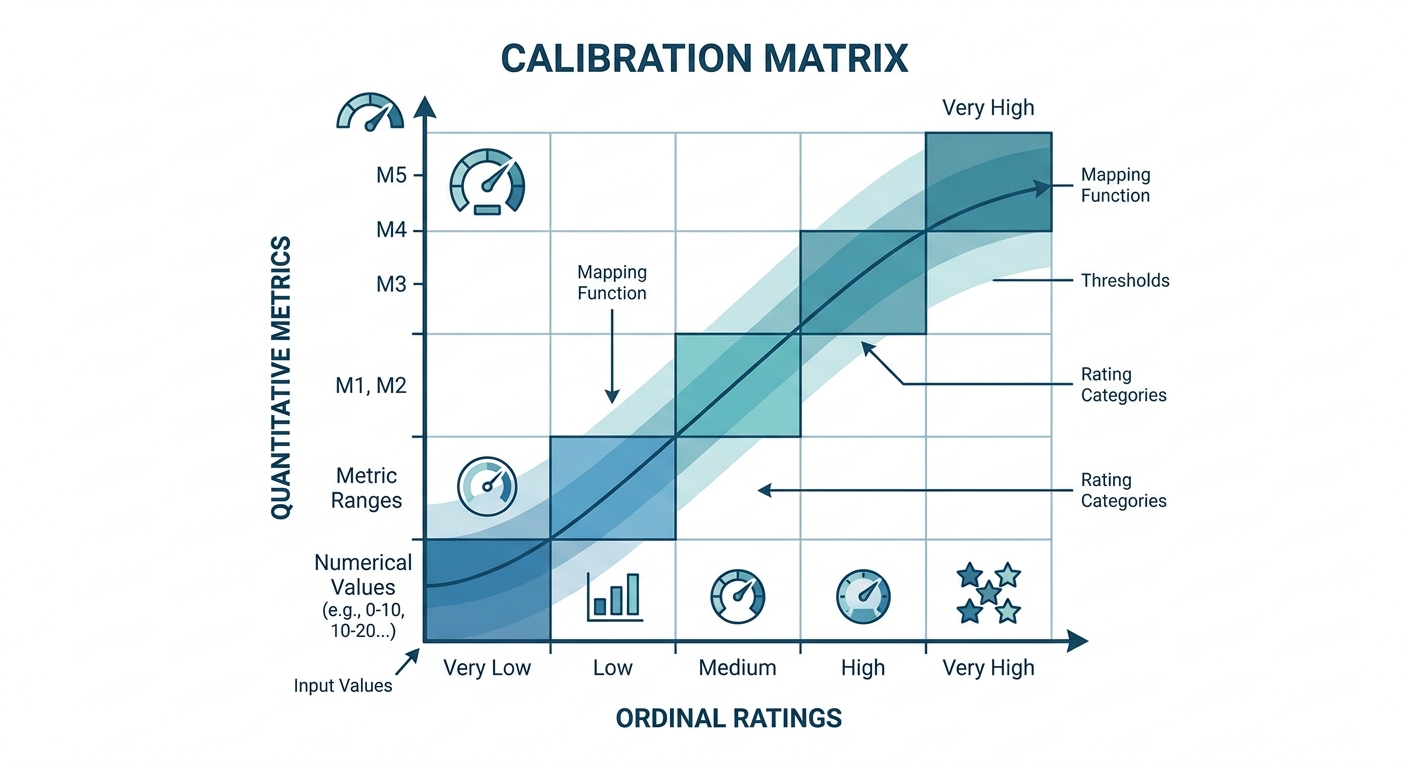
| Rating | Severity (\(S\)) Metric | Occurrence (\(O\)) Operational Frequency | Detection (\(D\)) Detection Capability |
|---|---|---|---|
| 10 | Unwarned catastrophic safety failure, injury, or severe regulatory breach | MTBF \(< 50\) hours (\(\text{Failure Rate } \lambda > 0.02/\text{hr}\)) | Non-detectable; no sensor, alarm, or inspection protocol exists |
| 7–9 | Major asset destruction; downtime \(> 24\) hours; high safety hazard | \(50 \le \text{MTBF} < 1{,}000\) hours | Manual off-line inspection required; long P-F interval gap |
| 4–6 | Partial yield loss; downtime \(2 \text{ to } 24\) hours; moderate repair costs | \(1{,}000 \le \text{MTBF} < 10{,}000\) hours | Periodic route-based condition monitoring (e.g., monthly vibration) |
| 1–3 | Minor inconvenience; downtime \(< 2\) hours; localized plant impact | MTBF \(\ge 10{,}000\) hours (\(\text{Failure Rate } \lambda \le 0.0001/\text{hr}\)) | Automated continuous inline sensors with immediate safety interlocks |
When calibrating Occurrence, failure rates (\(\lambda = 1 / \text{MTBF}\)) must be calculated using actual maintenance logs via an empirical Failure Rate Calculator.
For Detection scoring, teams must evaluate the relationship between inspection frequency and the P-F interval—the elapsed time between detectable potential failure (\(P\)) and functional failure (\(F\)). If the inspection interval exceeds the P-F interval, the detection capability is fundamentally flawed, requiring a rating of \(D \ge 8\) regardless of tool sophistication.
Step-by-Step Worked Numeric Example: High-Pressure Pump Analysis
Consider a critical high-pressure boiler feed pump in a cogeneration facility. The failure mode under evaluation is Mechanical Seal Face Degradation, resulting in fluid leakage and unannounced pump trips.
Step 1: Establish Baseline Scores
- Severity (\(S = 8\)): Flammable process fluid leak triggers localized fire suppression deployment and causes an estimated 14 hours of unscheduled production shutdown.
- Occurrence (\(O = 5\)): Plant history indicates a Mean Time Between Failures (MTBF) of 2,500 hours for standard carbon-face seals under abrasive fluid loading.
- Detection (\(D = 6\)): Fluid leakage is identified during operator walkdowns performed on weekly visual inspection routes.
$$\text{RPN}_{\text{baseline}} = S \cdot O \cdot D$$
$$\text{RPN}_{\text{baseline}} = 8 \cdot 5 \cdot 6 = 240$$
Step 2: Implement Engineering Mitigations
To reduce operational risk systematically, the reliability team implements two targeted engineering interventions:
- Material Upgrade (Occurrence Reduction): Upgrade seal faces to silicon carbide with an engineered API pressurized flush plan, extending MTBF beyond 15,000 hours (\(O_{\text{revised}} = 2\)).
- Instrumentation Improvement (Detection Improvement): Install continuous differential pressure sensors on the barrier fluid reservoir, wired directly into the SCADA safety interlock system (\(D_{\text{revised}} = 2\)).
Step 3: Calculate Mitigated Risk and Reduction Ratio
$$\text{RPN}_{\text{mitigated}} = S \cdot O_{\text{revised}} \cdot D_{\text{revised}}$$
$$\text{RPN}_{\text{mitigated}} = 8 \cdot 2 \cdot 2 = 32$$
The relative percentage reduction in risk across the asset life cycle is calculated as follows:
$$\text{Risk Reduction} = \left( \frac{\text{RPN}_{\text{baseline}} - \text{RPN}_{\text{mitigated}}}{\text{RPN}_{\text{baseline}}} \right) \cdot 100\%$$
$$\text{Risk Reduction} = \left( \frac{240 - 32}{240} \right) \cdot 100\% = 86.67\%$$
Figure 3: Risk reduction trajectory before and after failure mitigation
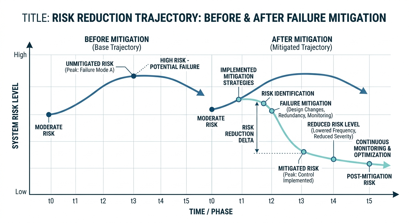
Cross-referencing this relative risk reduction with a Downtime Cost Calculator provides management with direct financial justification for capital expenditure on seal hardware and online instrumentation.
Establishing Governance and Alternative Prioritization Frameworks
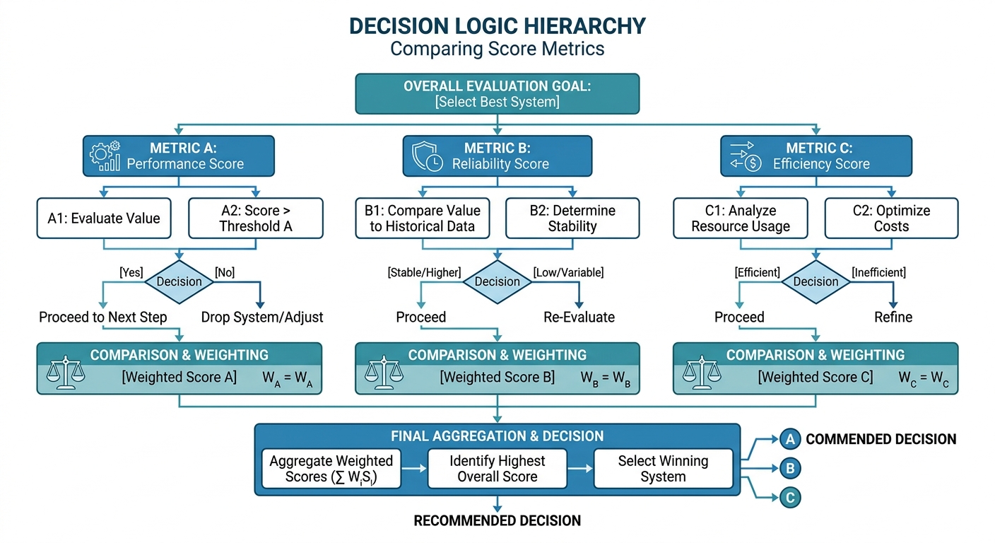
Relying on arbitrary cutoff thresholds (such as "mandatory engineering action for all items above 100") creates poor governance incentives. Engineering teams often artificially deflate ratings to avoid triggering administrative actions. Modern reliability programs replace arbitrary thresholds with structured priority logic.
Figure 4: Decision logic hierarchy comparing score metrics
High Severity First Policy
Under a High Severity First policy, any failure mode with \(S \ge 8\) mandates corrective action or explicit risk acceptance, regardless of the calculated RPN. For instance, a pressure vessel rupture mode with \(S=10, O=1, D=1 \implies \text{RPN}=10\) yields a deceptively low product score, yet demands engineering controls (e.g., burst discs, relief valves, structural containment) due to potential loss of life.
Action Priority (AP) Logic
The Action Priority framework replaces simple multiplication with qualitative logic tables that evaluate combinations of \(S\), \(O\), and \(D\) independently:
- High Priority (H): Highest priority for mitigation. The team must implement preventative controls or formally document why existing design controls are sufficient.
- Medium Priority (M): Action recommended. Teams should identify cost-effective risk reduction strategies or document operational safeguards.
- Low Priority (L): Low risk tier. Secondary review is optional; standard operating and maintenance procedures apply.
Using a Pareto Chart Tool, maintenance leaders can isolate the vital few failure modes driving facility risk and concentrate engineering resources where they yield maximum asset uptime.
Building a Sustainable Risk Prioritization Strategy
Constructing an effective risk priority system requires moving past simplistic multiplication tables and arbitrary RPN thresholds. By grounding Severity, Occurrence, and Detection scales in empirical MTBF calculations, quantified downtime costs, and P-F interval mechanics, engineering teams establish an accurate, repeatable risk profile. This structured methodology prevents high-consequence failure modes from hiding behind misleadingly low product scores while ensuring maintenance capital is deployed where it yields the highest return on asset reliability.
To streamline your facility's failure risk analysis and calculate critical asset metrics, explore the complete suite of analytical utilities available at ReliabilityCalc.com.