
When proposing capital expenditures for asset monitoring or preventive overhauls, engineering teams frequently face budget rejection from corporate finance. This friction rarely stems from poor engineering; it stems from unvalidated downtime cost estimates. Finance departments rightfully dismiss flat, anecdotal quotes like "$10,000 per hour."
Understating downtime cost starves high-return reliability initiatives of capital. Overstating it using top-line revenue numbers destroys engineering credibility during budget reviews. Quantifying downtime with financial precision bridges the gap between plant floor operations and corporate capital allocation.
Anatomy of Downtime Costs: Direct vs. Indirect Loss
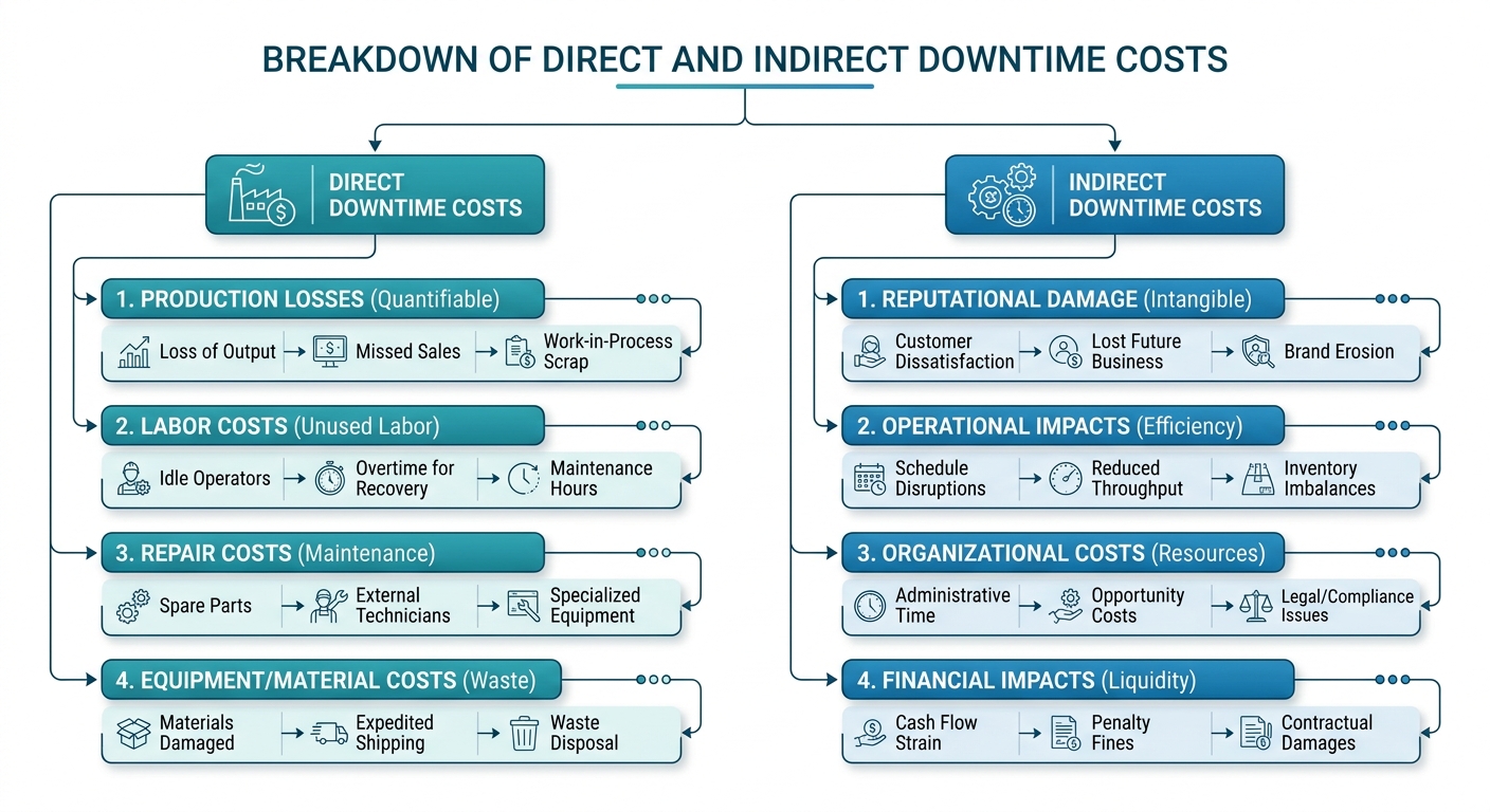
Calculating the true financial impact of an unscheduled stoppage requires separating operational losses into direct variable costs, fixed labor burdens, and indirect system-wide impacts. A primary analytical error is substituting gross lost revenue for true financial loss. Corporate controllers evaluate lost contribution margin—gross revenue minus raw material and variable utility costs unconsumed while the line is idle.
Direct downtime costs accrue immediately upon asset stoppage:
- Unrecovered operator labor burden
- Dedicated maintenance intervention labor
- Replacement parts and consumable materials
- Scrapped material stranded in processing zones
Indirect downtime costs propagate over time across the broader facility:
- Downstream process starvation that forces secondary assets idle
- Quality yield losses during thermal re-stabilization and line ramp-up
- Expedited freight fees and contractual service level agreement (SLA) penalties
Figure 1: Breakdown of direct and indirect downtime costs
To build a defensible financial model, classify each cost element by operational origin and variability:
| Cost Element | Category | Financial Calculation Basis | Sensitivity Factor |
|---|---|---|---|
| Lost Contribution Margin | Direct Variable | \(\text{Units Lost} \cdot (\text{Selling Price} - \text{Direct Material Cost})\) | Bottleneck asset utilization |
| Idle Direct Labor | Direct Fixed | \(\text{Downtime Hours} \cdot \text{Fully Burdened Labor Rate} \cdot \text{Headcount}\) | Redeployment efficiency |
| Scrap and Rework | Direct Variable | \((\text{Defective Units} \cdot \text{Unit Cost}) + \text{Rework Labor}\) | Re-stabilization duration |
| Maintenance Labor | Direct Variable | \(\text{Intervention Hours} \cdot \text{Burdened Overtime Rate} \cdot \text{Technicians}\) | Response time & parts availability |
| Customer SLA Penalties | Indirect Variable | Contractual breach penalties + Expedited freight | Safety stock buffer depth |
| Asset Degradation | Indirect Fixed | Premature depreciation via thermal/mechanical shock | Failure mode severity |
Financial models must distinguish bottleneck from non-bottleneck assets. Downtime on non-bottleneck equipment can often be absorbed by intermediate buffers without impacting plant output. Downtime on a primary bottleneck creates an unrecoverable net throughput loss.
Quantitative Framework for Total Hourly Downtime Cost
Total downtime cost (\(C_{\text{DT}}\)) for an unscheduled outage is defined as:
$$C_{\text{DT}} = (C_{\text{prod}} + C_{\text{labor}}) \cdot t_{\text{down}} + C_{\text{scrap}} + C_{\text{maint}} + C_{\text{pen}}$$
Where:
- \(C_{\text{prod}}\) is the hourly lost contribution margin (\(\$/\text{hour}\))
- \(C_{\text{labor}}\) is the combined hourly labor burden of idle operators and response technicians (\(\$/\text{hour}\))
- \(t_{\text{down}}\) is the total outage duration (\(\text{hours}\))
- \(C_{\text{scrap}}\) is the cost of damaged material and startup scrap (\(\\))
- \(C_{\text{maint}}\) is non-labor repair expense, including replacement parts and sub-contracted services (\(\\))
- \(C_{\text{pen}}\) is the sum of external logistics and contractual delay penalties (\(\\))
Hourly lost contribution margin (\(C_{\text{prod}}\)) depends on standard throughput (\(R\), in units/hour) and net contribution margin per unit (\(M\), in \(\$/\text{unit}\)):
$$C_{\text{prod}} = R \cdot M$$
When calculating \(M\), subtract unconsumed raw material costs from unit selling price, but retain fixed operating baseline costs.
Figure 2: Sequential stages of operational downtime recovery
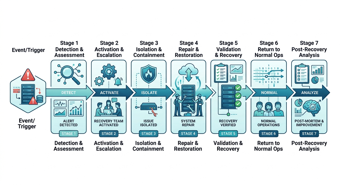
The duration term \(t_{\text{down}}\) extends beyond active repair time ("wrench time"). It encompasses four sequential phases: response lag, diagnostic isolation, physical repair, and functional re-commissioning. To evaluate baseline line losses before applying financial factors, use the OEE Calculator. To convert operational metrics directly into monetary figures, apply the Downtime Cost Calculator.
Worked Example: Automated Automotive Stamping Line
An automated stamping line supplying an OEM assembly plant suffers an unscheduled drive coupling failure.
Operational and Financial Parameters
- Standard Production Rate (\(R\)): \(120\text{ stampings/hour}\)
- Wholesale Selling Price: \(\$110.00/\text{unit}\)
- Direct Raw Material Cost (Steel): \(\$65.00/\text{unit}\)
- Net Contribution Margin (\(M\)): \(\$110.00 - \$65.00 = \$45.00/\text{unit}\)
- Idle Line Operators: \(8\text{ operators}\) @ \(\$35.00/\text{hour}\) (fully burdened)
- Response Maintenance Technicians: \(3\text{ specialists}\) @ \(\$55.00/\text{hour}\) (overtime rate)
- Outage Duration (\(t_{\text{down}}\)): \(2.5\text{ hours}\)
- Startup Scrap: \(15\text{ damaged panels}\) valued at full production cost (\(\$80.00/\text{unit}\))
- Replacement Mechanical Coupling: \(\$1{,}850.00\)
- Downstream Assembly Delay Penalty (\(C_{\text{pen}}\)): Fixed fee of \(\$1{,}200.00\)
Step 1: Hourly Lost Contribution Margin (\(C_{\text{prod}}\))
$$C_{\text{prod}} = 120\text{ units/hr} \cdot \$45.00/\text{unit} = \$5{,}400.00/\text{hour}$$
Step 2: Hourly Combined Labor Rate (\(C_{\text{labor}}\))
$$C_{\text{labor}} = (8 \cdot \$35.00) + (3 \cdot \$55.00) = \$280.00 + \$165.00 = \$445.00/\text{hour}$$
Step 3: Total Time-Dependent Cost
$$C_{\text{time}} = (C_{\text{prod}} + C_{\text{labor}}) \cdot t_{\text{down}} = (\$5{,}400.00 + \$445.00) \cdot 2.5\text{ hrs} = \$5{,}845.00 \cdot 2.5 = \$14{,}612.50$$
Step 4: Scrap and Spare Parts Costs (\(C_{\text{scrap}}\) and \(C_{\text{maint}}\))
$$C_{\text{scrap}} = 15\text{ units} \cdot \$80.00/\text{unit} = \$1{,}200.00$$
$$C_{\text{maint}} = \$1{,}850.00\text{ (coupling cost)}$$
Step 5: Total Outage Event Cost (\(C_{\text{DT}}\))
$$C_{\text{DT}} = C_{\text{time}} + C_{\text{scrap}} + C_{\text{maint}} + C_{\text{pen}}$$
$$C_{\text{DT}} = \$14{,}612.50 + \$1{,}200.00 + \$1{,}850.00 + \$1{,}200.00 = \$18{,}862.50$$
This \(2.5\text{-hour}\) failure cost \(\$18{,}862.50\), representing an effective hourly downtime cost of:
$$\text{Effective Hourly Downtime Rate} = \frac{\$18{,}862.50}{2.5\text{ hrs}} = \$7{,}545.00/\text{hour}$$
Tracking only maintenance labor and parts—a common accounting mistake—reports an event cost of just \((\$165.00 \cdot 2.5) + \$1{,}850.00 = \$2{,}262.50\). This understates the business impact by \(88.0\%\), obscuring the true ROI of predictive maintenance investments.
Capital Project Justification and Payback Analysis
To secure approval for condition monitoring systems or asset redesigns, link expected failure rate reductions directly to annual downtime savings.
First, establish baseline unreliability costs. If an asset has a failure rate (\(\lambda\)) of \(4.8\text{ failures/year}\) and a Mean Time to Repair (\(MTTR\)) of \(2.5\text{ hours}\), total annual unplanned downtime is \(12.0\text{ hours}\). Validate these baselines using the MTTR Calculator and Availability Calculator.
Consider a proposed online vibration monitoring system costing \(\$24{,}000\) to install, plus \(\$3{,}000/\text{year}\) in software licensing. Reliability models project that early fault detection will shift \(75\%\) of catastrophic failures (\(3.6\text{ events/year}\)) to planned off-shift PMs.
Figure 3: Capital expenditure payback curve versus downtime reduction
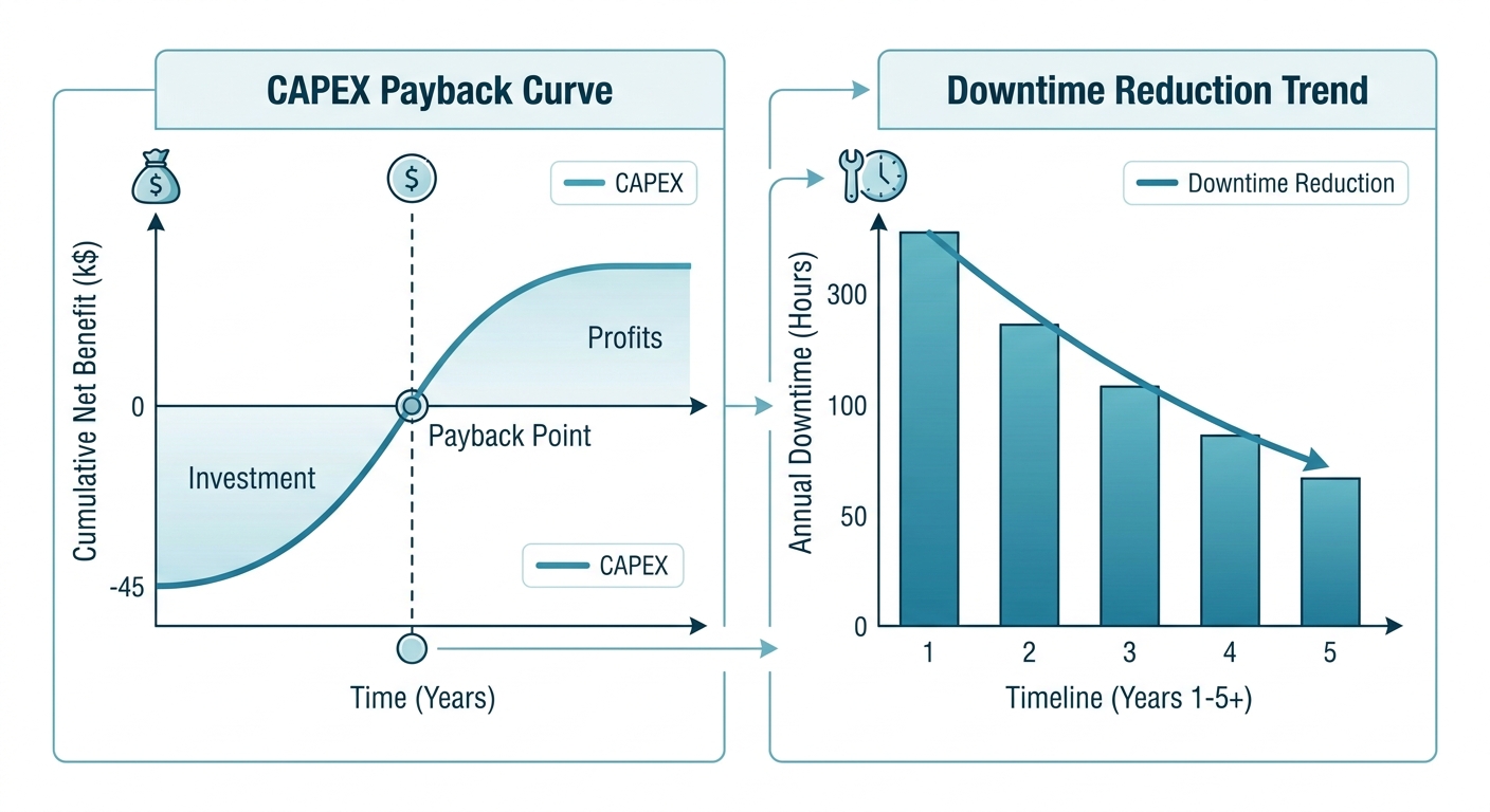
Off-shift planned maintenance eliminates contractual penalties (\(C_{\text{pen}} = \$0\)), prevents production loss (\(C_{\text{prod}} = \$0\)), reduces startup scrap by \(80\%\), and lowers repair duration (\(MTTR\)) from \(2.5\) to \(1.0\text{ hour}\).
Cost Comparison per Incident
- Unplanned Outage Cost: \(\$18{,}862.50\)
- Planned PM Cost:
- Production Margin Loss (\(C_{\text{prod}}\)): \(\$0.00\)
- Technician Labor (\(2\text{ techs} \cdot 1.0\text{ hr} \cdot \$50.00/\text{hr}\)): \(\$100.00\)
- Spare Parts (reduced damage scope): \(\$850.00\)
- Startup Scrap (\(3\text{ panels} \cdot \$80.00\)): \(\$240.00\)
- Penalty (\(C_{\text{pen}}\)): \(\$0.00\)
- Total Planned Event Cost: \(\$1{,}190.00\)
Converting \(3.6\text{ events/year}\) from unplanned outages to planned PMs yields gross annual savings of:
$$\text{Savings}_{\text{gross}} = 3.6 \cdot (\$18{,}862.50 - \$1{,}190.00) = 3.6 \cdot \$17{,}672.50 = \$63{,}621.00/\text{year}$$
Subtracting the \(\$3{,}000\) recurring software license leaves a net annual benefit of \(\$60{,}621.00/\text{year}\).
$$\text{Simple Payback Period} = \frac{\text{Initial Capital Investment}}{\text{Net Annual Cash Benefit}} = \frac{\$24{,}000}{\$60{,}621.00} = 0.396\text{ years } (\approx 4.75\text{ months})$$
Framing capital requests with this degree of financial rigor converts maintenance proposals from overhead expenses into high-yield business cases.
Conclusion
Justifying reliability capital requires converting operational stoppage metrics into rigorous contribution margin losses, burdened labor costs, and penalty structures. Quantifying these variables equips engineers to present capital projects in terms executive leadership respects. For interactive modeling tools, asset templates, and financial calculation engines, visit ReliabilityCalc.com.