
A continuous packaging facility operates 24/7 with a crew of sixteen multi-craft technicians. The Computerized Maintenance Management System (CMMS) reports 94% schedule compliance. Simultaneously, the work order backlog expands by forty hours each week, overtime exceeds 18%, and mean downtime after interventions continues to climb.
This paradox is common: high schedule compliance often masks low labor productivity. Tracking asset utilization alone ignores the efficiency of the human capital maintaining those assets. Just as physical equipment availability, performance, and quality are evaluated through an OEE Calculator, workforce performance requires an equivalent operational framework: Overall Labor Effectiveness (OLE).
In industrial maintenance, OLE does not monitor personal worker hustle. It exposes systemic operational friction—including parts-kitting deficits, incomplete job plans, transit waste, and craft-induced rework—that degrades technical capacity.
Figure 1: Three pillars of maintenance labor effectiveness
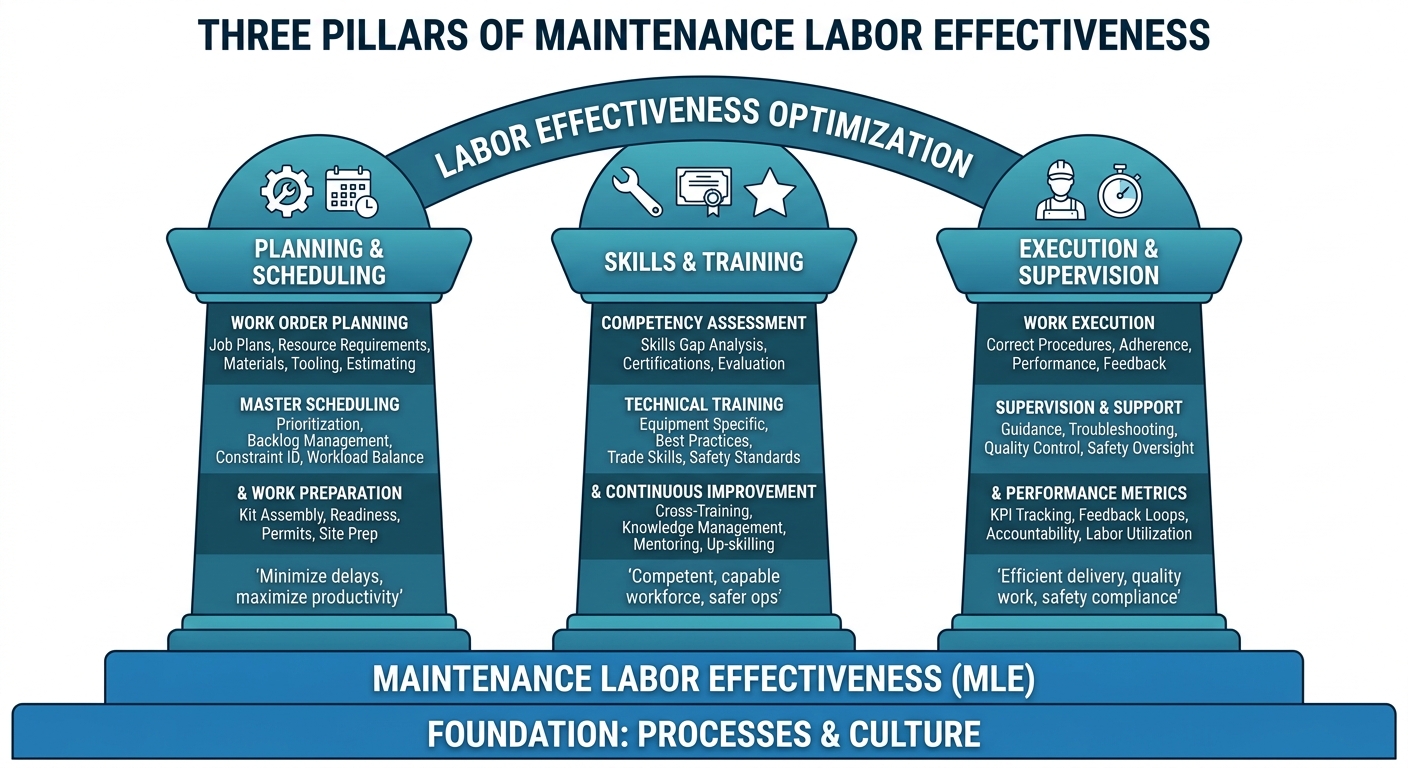
The Triad of Maintenance Workforce Efficiency
Overall Labor Effectiveness breaks technical labor utilization into three discrete, measurable components: Availability (\(A_L\)), Performance (\(P_L\)), and Quality (\(Q_L\)).
$$OLE = A_L \times P_L \times Q_L$$
Each dimension isolates a distinct failure mode within maintenance operations and job planning workflows.
1. Labor Availability (\(A_L\))
Labor Availability measures the proportion of scheduled payroll time that technicians directly execute physical maintenance tasks—frequently referred to as "wrench time." It isolates administrative overhead, permit bottlenecks, and material logistics delays from direct work execution.
$$A_L = \frac{\text{Direct Work Execution Hours}}{\text{Gross Scheduled Hours}} = \frac{H_{\text{actual}}}{H_{\text{gross}}}$$
Availability losses stem from operational friction prior to or between work order executions:
- Delays in Lock-Out/Tag-Out (LOTO) verification and safe-work permit sign-offs
- Travel time across large geographic footprints or multi-floor production structures
- Staging bottlenecks at the central tool crib or storeroom parts counter
- Non-maintenance administrative tasks, unstructured shift handovers, and compliance briefings
If an eight-hour shift includes two hours of permit coordination, storeroom queues, and travel, the technical availability of that asset resource is capped at 75% before any mechanical work begins.
2. Labor Performance (\(P_L\))
Labor Performance benchmarks execution velocity against planned standards. It evaluates the ratio of standard planned hours (earned hours) to the actual direct hours spent completing work packages.
$$P_L = \frac{\text{Standard Planned Hours Delivered}}{\text{Actual Direct Work Hours Expended}} = \frac{H_{\text{standard}}}{H_{\text{actual}}}$$
Standard hours represent realistic task durations established by maintenance planners, historical work studies, or engineered standard job plans. Performance losses indicate execution impediments during the job:
- Missing, obsolete, or ambiguous technical documentation and schematics
- Inadequate or uncalibrated specialized rigging and precision alignment tooling
- Unexpected equipment conditions (e.g., corroded fasteners, piping misalignment, or undocumented field modifications)
- Craft skill mismatches relative to technical task requirements
Pace variances directly affect asset turnaround times, which reliability teams can evaluate using an MTTR Calculator.
3. Labor Quality (\(Q_L\))
Labor Quality represents the proportion of maintenance interventions completed without triggering infant mortality, procedural omissions, or premature re-failure within a defined operational window (typically 7 to 30 days post-intervention).
$$Q_L = \frac{H_{\text{standard}} - H_{\text{rework}}}{H_{\text{standard}}} = \frac{H_{\text{quality}}}{H_{\text{standard}}}$$
Quality losses manifest as post-maintenance asset instability:
- Immediate startup aborts caused by misaligned interlocks, uncalibrated instrumentation, or closed isolation valves
- Installation defects, such as improper bearing clearances, overtightened mechanical packings, or missing dynamic balance checks
- Early-life component fatigue driven by uncorrected soft-foot or precision alignment failures
Completing an overhaul in half the estimated time yields high individual performance. However, if unverified alignment causes the mechanical seal to fail 48 hours later, the work produced negative net reliability value.
Figure 2: Maintenance labor loss waterfall breakdown
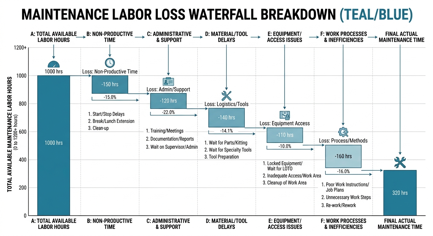
Step-by-Step Calculation: Mechanical Reliability Crew
The following calculation evaluates a mechanical maintenance crew maintaining an automated chemical processing facility over a continuous four-week cycle.
Baseline Parameters
- Scheduled Headcount: \(N = 8\text{ mechanical technicians}\)
- Shift Duration: \(40\text{ hours/week per technician}\)
- Time Horizon: \(T = 4\text{ weeks}\) (160 nominal hours per technician)
- Gross Scheduled Labor Hours:
$$H_{\text{gross}} = 8 \times 160 = 1{,}280\text{ hours}$$
Step 1: Compute Labor Availability (\(A_L\))
CMMS time-card logs, facility badging, and work order audit records account for non-direct labor allocations over the period:
- Mandatory safety meetings and compliance training: \(110\text{ hours}\)
- Storeroom parts retrieval and parts-kitting delays: \(145\text{ hours}\)
- Operations permit sign-offs and LOTO execution: \(95\text{ hours}\)
- Inter-facility transit and rigging mobilization: \(70\text{ hours}\)
Total logistical and administrative loss:
$$H_{\text{loss, avail}} = 110 + 145 + 95 + 70 = 420\text{ hours}$$
Actual direct hours applied to physical assets:
$$H_{\text{actual}} = H_{\text{gross}} - H_{\text{loss, avail}} = 1{,}280 - 420 = 860\text{ hours}$$
Labor Availability:
$$A_L = \frac{860}{1{,}280} \approx 0.6719\text{ (67.19\%)}$$
Step 2: Compute Labor Performance (\(P_L\))
Across the 860 hours of direct tool time, the crew executed planned preventive maintenance tasks, precision rebuilds, and routine corrective work orders. Planned baseline durations stored in the CMMS job library total:
- Standard Planned Hours Delivered: \(H_{\text{standard}} = 740\text{ hours}\)
Labor Performance:
$$P_L = \frac{740}{860} \approx 0.8605\text{ (86.05\%)}$$
The variance (\(860 - 740 = 120\text{ hours}\)) reflects time lost to unforeseen field complications, incomplete task procedures, and improvised tooling.
Step 3: Compute Labor Quality (\(Q_L\))
Reliability engineering tracks asset performance for 30 days following work order closure. CMMS records reveal two primary rework interventions tied to craft quality errors:
- Dynamic balancing and alignment corrections on three slurry pumps: \(48\text{ hours}\)
- Flange reseating and gasket replacement due to uneven bolt torque: \(22\text{ hours}\)
Total rework hours generated:
$$H_{\text{rework}} = 48 + 22 = 70\text{ hours}$$
Net effective reliability hours:
$$H_{\text{quality}} = 740 - 70 = 670\text{ hours}$$
Labor Quality:
$$Q_L = \frac{670}{740} \approx 0.9054\text{ (90.54\%)}$$
Step 4: Calculate Compound Overall Labor Effectiveness
Multiplying the three operational factors yields the net OLE score:
$$OLE = A_L \times P_L \times Q_L$$
$$OLE = \left(\frac{860}{1{,}280}\right) \times \left(\frac{740}{860}\right) \times \left(\frac{670}{740}\right) = \frac{670}{1{,}280} \approx 0.5234\text{ (52.34\%)}$$
(Note: Multiplying rounded values yields \(0.6719 \times 0.8605 \times 0.9054 = 0.5235\), or 52.35%.)
Out of 1,280 funded payroll hours, only 670 hours converted into durable, defect-free maintenance output. The largest capacity leak is not trade execution pace, but the 420 hours lost to logistical, administrative, and staging friction.
Figure 3: Correlation between workforce performance and MTTR
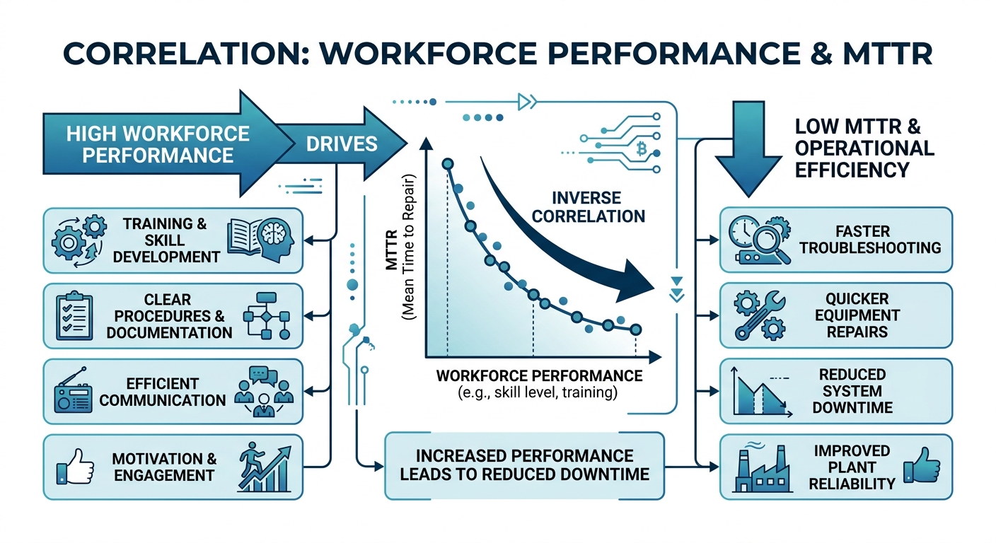
Diagnostic Matrix: Isolating Maintenance Delivery Losses
When technicians spend less than half their scheduled shift applying technical skills directly to assets, hiring additional staff simply amplifies existing process waste. Use a Pareto Chart Tool to identify and prioritize the root causes dragging down OLE components.
| Dimension | Primary Failure Mode | Underlying Root Cause | Corrective Engineering Action |
|---|---|---|---|
| Availability | Technicians waiting at storeroom counters | Reactive staging; uncoordinated bills of materials | Implement mandatory advance kitting for all scheduled tasks 24 hours prior to release |
| Availability | Transit waste and logistical delays | Centralized tooling in expansive facilities | Deploy decentralized satellite cribs for consumables, rigging gear, and fast-moving hardware |
| Availability | Prolonged safe-work permit approvals | Disconnected safety protocols and planning loops | Pre-populate LOTO procedures and permit documentation directly in CMMS job plans |
| Performance | Field execution time exceeding estimates | Inaccurate task sequences and non-standard tooling | Audit job plans; define clear step-by-step procedures, tolerances, and tooling requirements |
| Performance | Assembly stalls from field interferences | Incomplete records of prior equipment modifications | Establish a post-work feedback loop requiring redline updates to mechanical drawings |
| Quality | Early failure of rotating equipment | Absence of documented assembly tolerances | Enforce precision assembly checklists covering runout, cold-alignment targets, and soft-foot |
| Quality | Premature hydraulic and bearing failures | Contamination during fluid handling and assembly | Enforce sealed transfer containers, clean-break couplings, and ISO 4406 fluid standards |
Financial and Operational Impact
Depressed craft productivity directly damages plant financial performance. Low Availability forces corrective tasks to take longer, inflating Mean Time to Repair (MTTR) and extending production outages. The cost of this downtime can be modeled with a Downtime Cost Calculator.
Consider the cascading costs of poor Labor Quality. If an improperly torqued mechanical seal fails on a critical chemical pump:
- The initial 16-hour overhaul is lost.
- A secondary 16-hour repair must be performed under urgent, higher-cost conditions.
- Consumable assets (mechanical seal faces, gaskets, synthetic lubricant) are destroyed.
- Production volume is sacrificed while the line remains offline.
Conversely, lifting Availability from 67% to 80% through advance parts kitting and digital LOTO workflows restores 164 wrench hours per month for an 8-person crew—the operational equivalent of adding one full-time technician without increasing headcount.
Optimizing Workforce Performance
Overall Labor Effectiveness replaces subjective assessments of craft productivity with an objective engineering standard. A drop in Availability points to structural failures in planning, scheduling, or storeroom logistics. A drop in Performance highlights gaps in technical documentation, tooling, or task scoping. A drop in Quality demands immediate revision of assembly specifications, precision standards, and sign-off criteria.
Treating maintenance craft hours as finite engineering assets allows reliability leaders to remove administrative friction, eliminate rework loops, and sustain operational throughput. To evaluate labor utilization, downtime exposure, and physical asset metrics across your plant, explore the engineering models at ReliabilityCalc.com.