In the pursuit of operational excellence, maintenance departments are often trapped between the inefficiency of premature replacement and the high cost of catastrophic failure. While high-level metrics like Mean Time Between Failures (MTBF) offer a snapshot of population performance, they are fundamentally "memoryless" and fail to account for the actual physics of failure. To accurately predict when a component will reach its end-of-life, reliability engineers utilize Weibull analysis. Developed by Waloddi Weibull, this statistical method is the cornerstone of Life Data Analysis (LDA) because it can model a diverse range of failure distributions using a remarkably small number of data points.
For professionals operating under ISO 55000 asset management standards or IEC 60300 dependability guidelines, Weibull analysis is a technical necessity. It allows engineers to distinguish between infant mortality, random chance, and wear-out phases, directly informing whether a strategy should prioritize quality control, condition monitoring, or hard-time replacement.
The Three Pillars of the Weibull Distribution
The utility of the Weibull distribution lies in its mathematical flexibility. By adjusting its parameters, the distribution can emulate other statistical models, including the Exponential, Normal, and Lognormal distributions. Mastery of these three parameters is essential when using a Weibull Analysis Calculator to interpret field data.
1. The Shape Parameter (Beta, β)
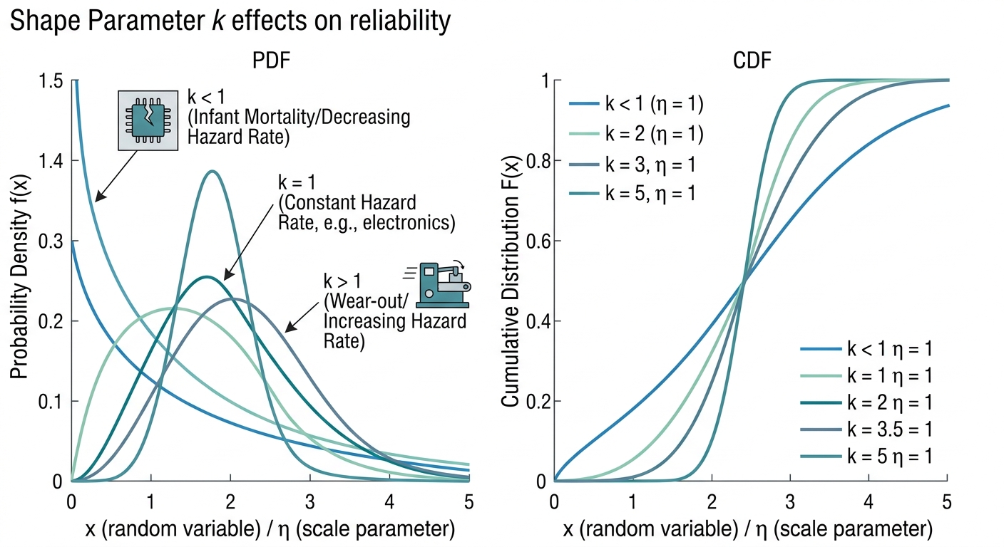
The shape parameter, \(\beta\), is the most critical output of the analysis as it defines the failure mechanism.
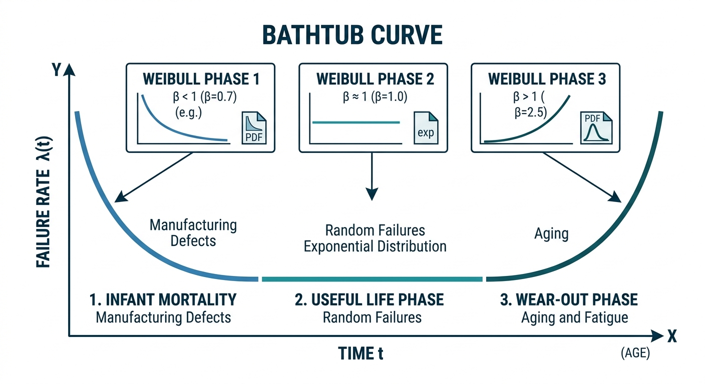
- \(\beta < 1\) (Infant Mortality): The failure rate decreases over time. This typically indicates "burn-in" issues, manufacturing defects, or installation errors.
- \(\beta = 1\) (Random Failure): The failure rate is constant. This reduces to the Exponential distribution, where failures are caused by external stressors rather than aging. In this phase, reliability can be accurately modeled using a standard MTBF Calculator.
- \(\beta > 1\) (Wear-out): The failure rate increases over time. This is the domain of fatigue, corrosion, and mechanical degradation. A \(\beta\) between 1.5 and 4.0 often indicates fatigue, while \(\beta > 4.0\) suggests rapid wear-out or chemical decomposition.
2. The Scale Parameter (Eta, η)
Also known as the "Characteristic Life," \(\eta\) represents the point in time at which 63.2% of the population is expected to have failed, regardless of the \(\beta\) value. Unlike the arithmetic mean, which can be heavily skewed by outliers, \(\eta\) provides a robust measure of the life of a component within its specific failure mode.
3. The Location Parameter (Gamma, γ)
The location parameter shifts the distribution along the time axis, representing a "failure-free" period. For instance, if a component is designed with a guaranteed minimum life of 500 hours, \(\gamma\) would be 500. In most industrial reliability models, \(\gamma\) is assumed to be zero, implying that the risk of failure begins immediately at \(t=0\).
Figure 1: Weibull distribution shape parameter effects
| Parameter | Symbol | Engineering Significance | Impact on Maintenance Strategy |
|---|---|---|---|
| Shape | \(\beta\) | Defines failure mode (Infant vs. Wear-out) | Determines if PM is technically feasible |
| Scale | \(\eta\) | Defines "Characteristic Life" (63.2% point) | Drives spare parts and logistics planning |
| Location | \(\gamma\) | Defines "Failure-Free" period | Validates warranty and design minimums |
Data Preparation and Parameter Estimation
Performing a valid Weibull analysis requires high-quality "Time-to-Failure" (TTF) data. In practice, this data is often "censored." Right-censored data, or suspensions, occurs when a component is removed from service before failure or remains operational at the time of analysis. Ignoring these suspensions introduces a "pessimistic bias," underestimating the true reliability of the asset.
The two primary methods for estimating parameters are Rank Regression (Least Squares) and Maximum Likelihood Estimation (MLE). While MLE is the industry standard for large datasets and complex censoring (as outlined in MIL-HDBK-338B), Rank Regression remains highly effective for the small sample sizes (\(n < 30\)) frequently encountered in specialized equipment testing.
Figure 2: Linearized Weibull probability plot for parameter estimation
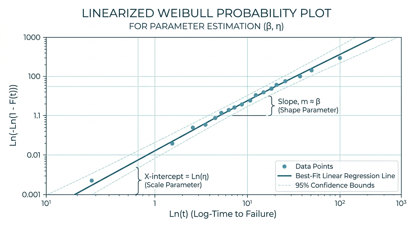
When TTF data is plotted on Weibull probability paper—utilizing a double-logarithmic scale for the y-axis—the distribution appears as a straight line. The slope of this line represents \(\beta\), while the intercept is used to derive \(\eta\). This visualization is essential for identifying "sub-populations," such as when a single batch of components exhibits two distinct failure modes due to a manufacturing shift.
Worked Example: Bearing Fatigue Analysis
Consider a reliability engineer investigating the failure of five high-speed pump bearings. The objective is to determine the failure mode and calculate the Reliability of the remaining units at the 2,000-hour mark.
Input Data (Hours to Failure):
- 1,200 hrs
- 1,550 hrs
- 1,800 hrs
- 2,100 hrs
- 2,450 hrs
Step 1: Rank the Data
Order the failures from shortest to longest life (\(i=1\) to \(n=5\)).
Step 2: Calculate Median Ranks
Using Benard’s approximation, \(F(t) = (i - 0.3) / (n + 0.4)\), we determine the cumulative failure probability:
- \(F(1) = (1 - 0.3) / 5.4 = 0.1296\)
- \(F(2) = (2 - 0.3) / 5.4 = 0.3148\)
- \(F(3) = (3 - 0.3) / 5.4 = 0.5000\)
- \(F(4) = (4 - 0.3) / 5.4 = 0.6852\)
- \(F(5) = (5 - 0.3) / 5.4 = 0.8704\)
Step 3: Linear Transformation
The Weibull Cumulative Distribution Function (CDF) is \(F(t) = 1 - e^{-(t/\eta)^\beta}\). To perform linear regression, we transform the equation into the form \(y = mx + c\):
$$\ln(-\ln(1 - F(t))) = \beta \ln(t) - \beta \ln(\eta)$$
Where \(y = \ln(-\ln(1 - F(t)))\) and \(x = \ln(t)\).
Step 4: Regression Results
Performing a least-squares regression on the transformed \(x\) and \(y\) values yields:
- \(\beta \approx 3.74\)
- \(\ln(\eta) \approx 7.607 \rightarrow \eta \approx 2,012\) hours
Step 5: Interpretation
A \(\beta\) of 3.74 confirms a "Wear-out" mode, specifically characteristic of material fatigue. This indicates that the Failure Rate is increasing rapidly, making preventative maintenance (PM) highly effective.
To calculate the reliability at 2,000 hours:
$$R(2000) = e^{-(2000/2012)^{3.74}}$$
$$R(2000) = e^{-(0.994)^{3.74}} = e^{-0.9778} \approx 0.376$$
There is only a 37.6% probability that a bearing will survive to 2,000 hours. The engineer should schedule replacements significantly before this interval to prevent unplanned downtime.
Figure 3: Bathtub curve relationship to Weibull phases
Strategic Application in Asset Management
Weibull analysis provides the objective evidence required to transition from reactive to proactive maintenance. By identifying the \(\beta\) value, managers can align their interventions with the physical reality of the asset:
- For \(\beta \approx 1\): Scheduled replacements are mathematically ineffective and wasteful. Resources should be redirected toward condition monitoring (vibration analysis, oil sampling) or a run-to-fail strategy for non-critical assets.
- For \(\beta > 2\): Scheduled restoration or replacement is the optimal strategy. Engineers can calculate the "Optimum Replacement Interval" to balance the cost of planned maintenance against the significantly higher cost of an in-service failure.
- For \(\beta < 1\): Maintenance is often the problem, not the solution. High infant mortality suggests issues in the supply chain, storage conditions, or installation quality. Performing PM in this phase will actually increase the total failure rate due to "maintenance-induced" infant mortality.
Integrating these outputs into a System Reliability Calculator allows for the modeling of complex, redundant systems. If a system utilizes parallel pumps and Weibull analysis shows both are entering a wear-out phase, the probability of a total system outage increases non-linearly, necessitating immediate intervention.
Conclusion
Weibull analysis transforms disparate failure dates into a predictive roadmap. By quantifying the shape and scale of failure distributions, reliability engineers can move beyond the simplistic assumptions of MTBF and develop strategies that reflect the true physical state of their equipment. Whether managing a fleet of heavy machinery or high-precision electronics, the precision of the Weibull distribution ensures that maintenance is performed at the point of maximum economic and operational value. To streamline these complex calculations and ensure the integrity of your data modeling, utilize the professional-grade tools available at ReliabilityCalc.com.