
Unplanned bearing failures on a critical 250 kW boiler feed pump trigger immediate plant trips, incurring downtime costs exceeding $30,000 per hour. Time-based preventive maintenance (PM) attempts to mitigate this risk by replacing components at static calendar intervals. However, schedule-based overhauls introduce infant mortality risks through reassembly errors, misalignment, and lubricant contamination, while remaining incapable of preventing random stress failures between service intervals.
Condition-based monitoring replaces arbitrary maintenance intervals with real-time asset health tracking. By capturing physical degradation signatures—such as high-frequency acoustic emissions, structural vibration, oil contamination, and thermal anomalies—reliability engineers intervene precisely when asset health breaches critical operational limits, preventing secondary damage and catastrophic downtime.
Sensor Selection and Data Modalities for Condition Monitoring
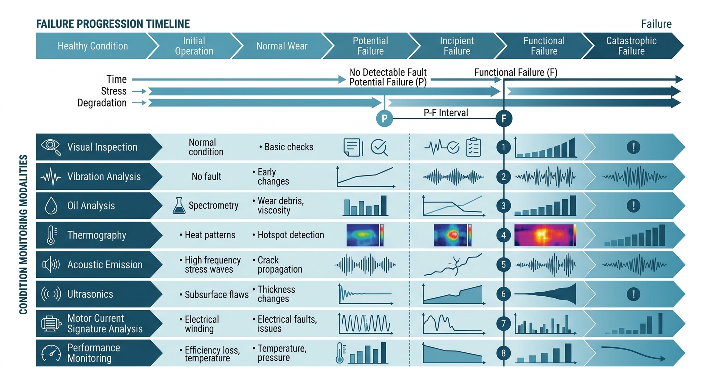
Implementing a condition monitoring program requires mapping specific failure mechanisms to high-sensitivity sensing technologies. No single parameter captures every degradation pathway across mechanical, electrical, and hydraulic sub-systems.
A complete monitoring program pairs asset failure modes—identified via Failure Modes, Effects, and Criticality Analysis (FMECA)—with complementary diagnostic sensors. For rolling element bearings, failure progresses predictably: subsurface micro-spalling releases high-frequency acoustic stress waves, followed by high-frequency impact acceleration, discrete defect frequencies in the velocity spectrum, localized thermal elevation, and structural clearance loss.
| Sensing Modality | Primary Failure Modes Detected | Lead Time to Failure | Typical Asset Applications |
|---|---|---|---|
| Vibration Analysis | Dynamic unbalance, angular/parallel misalignment, bearing defects, gear mesh wear, structural looseness | Weeks to Months | Turbomachinery, gearboxes, centrifugal pumps, industrial fans |
| Oil Analysis / Tribology | Viscosity degradation, particle contamination, additive depletion, metallic wear debris | Months | Reciprocating engines, hydraulic systems, closed gear drives |
| Infrared Thermography | High contact resistance, insulation breakdown, refractory degradation, abnormal friction | Days to Weeks | Electrical switchgear, power transformers, steam traps, motor control centers |
| Motor Current Signature Analysis (MCSA) | Cracked rotor bars, turn-to-turn short circuits, dynamic/static air gap eccentricity | Weeks to Months | High-voltage induction motors, submerged pump drives |
| Acoustic Emission (AE) | Micro-cracking, friction, fluid leakage, subsurface contact fatigue | Months | High-pressure piping, slow-rotating bearings (\(< 10 \text{ RPM}\)) |
Selecting an inappropriate modality creates dangerous diagnostic blind spots. Applying standard velocity transducers (\(\text{10 Hz}\) to \(\text{1 kHz}\)) to a conveyor bearing rotating at \(5 \text{ RPM}\) fails to register transient impact energy until failure occurs. Low-speed applications require high-frequency stress wave analysis or acoustic emission tracking. To systematically map asset failure modes to diagnostic metrics during risk evaluations, engineers use an FMEA Tool.
Figure 1: Condition monitoring modalities across failure progression
Signal Processing and Feature Extraction Techniques
Raw sensor time-series data must be processed into diagnostic metrics. In vibration monitoring, time-domain parameters quantify overall energy but lack fault isolation capabilities. Root Mean Square (RMS) acceleration measures total dynamic signal power:
$$a_{\text{RMS}} = \sqrt{\frac{1}{N} \sum_{i=1}^{N} x_i^2}$$
RMS acceleration tracks general severity but stays insensitive to early rolling element defects, where localized impacts create short-duration, high-amplitude peaks without changing total signal energy. To capture early transient impacts, engineers track Crest Factor (\(C_F\)) and Kurtosis (\(K\)):
$$C_F = \frac{x_{\text{peak}}}{a_{\text{RMS}}}$$
$$K = \frac{\frac{1}{N} \sum_{i=1}^{N} (x_i - \bar{x})^4}{\left(\frac{1}{N} \sum_{i=1}^{N} (x_i - \bar{x})^2\right)^2}$$
A healthy Gaussian amplitude distribution yields a Kurtosis value of \(3.0\). Micro-spalling on a bearing race causes localized shock impacts, raising Kurtosis to \(6.0\) or higher. As wear spreads across the bearing track, transient impacts blend into background noise, causing Kurtosis to return toward \(3.0\) near complete failure. Consequently, time-domain indicators must be coupled with Fast Fourier Transform (FFT) spectral analysis and envelope demodulation.
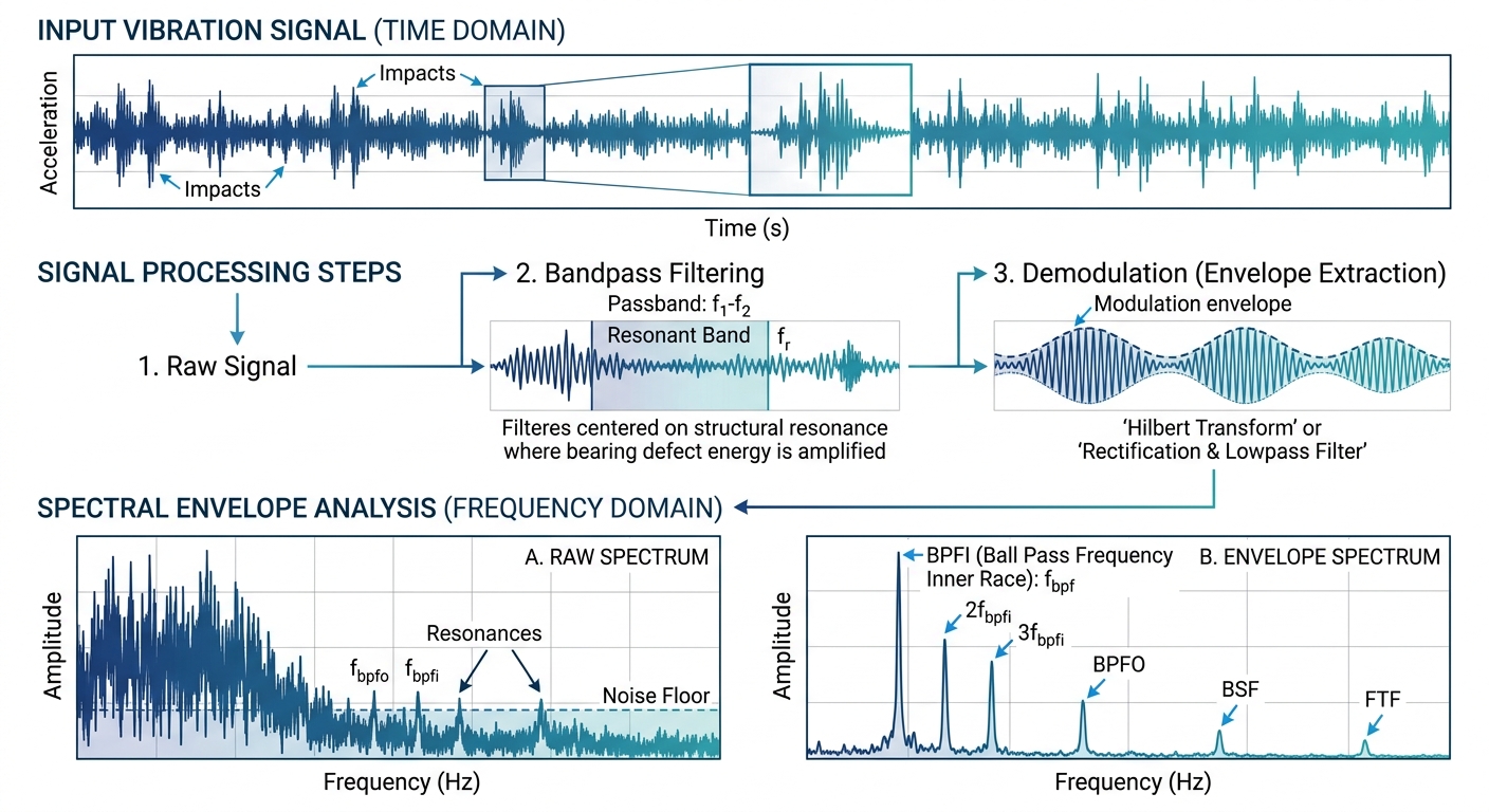
Envelope demodulation filters low-frequency rotational dynamics, isolating the high-frequency structural resonances excited by bearing impacts. The resulting demodulated spectrum yields discrete fault frequencies:
- Ball Pass Frequency Outer Race (BPFO): \(f_{\text{BPFO}} = \frac{N_b}{2} f_r \left(1 - \frac{d}{D} \cos\theta\right)\)
- Ball Pass Frequency Inner Race (BPFI): \(f_{\text{BPFI}} = \frac{N_b}{2} f_r \left(1 + \frac{d}{D} \cos\theta\right)\)
Where \(N_b\) is the number of rolling elements, \(f_r\) is running speed, \(d\) is ball diameter, \(D\) is pitch diameter, and \(\theta\) is contact angle. Trending these frequency amplitudes tracks localized wear propagation.
Figure 2: Spectral envelope analysis revealing bearing defect frequencies
Quantitative ROI Calculation for Condition Monitoring
Justifying capital investments in edge sensors, telemetry gateways, and diagnostic software requires a clear financial evaluation.
Consider an industrial facility operating 8 critical overhung process pumps driven by \(350 \text{ kW}\) motors.
Historical Baseline Parameters
- Fleet size (\(N_{\text{assets}}\)): \(8 \text{ pumps}\)
- Historical failure rate (\(\lambda_{\text{hist}}\)): \(0.45 \text{ failures/asset-year}\)
- Total annual unplanned failures (\(N_{\text{fail}}\)): \(8 \cdot 0.45 = 3.6 \text{ failures/year}\)
- Average unplanned failure cost (\(C_{\text{unplanned}}\)): \(\$28{,}000\) (includes secondary mechanical seal and impeller damage, expedited freight, overtime labor, and lost throughput)
- Baseline annual repair expenditure:
$$Cost_{\text{base}} = 3.6 \cdot \$28{,}000 = \$100{,}800/\text{year}$$
To quantify economic losses from production interruptions, model asset outage scenarios with the Downtime Cost Calculator.
Condition Monitoring Implementation Parameters
- Hardware, sensor installation, and gateway setup: \(\$32{,}000\) amortized over 5 years (\(\$6{,}400/\text{year}\))
- Annual software license and cloud analytics subscription: \(\$7{,}200/\text{year}\)
- Annual monitoring labor and data auditing: \(\$4{,}800/\text{year}\)
- Total annualized program cost (\(C_{\text{pdm}}\)):
$$C_{\text{pdm}} = \$6{,}400 + \$7{,}200 + \$4{,}800 = \$18{,}400/\text{year}$$
Operating Cost Parameters
- Planned repair cost under early PdM detection (\(C_{\text{planned}}\)): \(\$6{,}500\) (scheduled bearing replacement, zero secondary impeller damage, standard labor rate)
- PdM diagnostic effectiveness (\(\eta\)): \(85\%\) (85% of impending failures caught early; 15% manifest as sudden catastrophic events uncaught by sensors)
Financial Step-by-Step Calculation
- Calculate annual planned vs. unplanned repair counts:
$$N_{\text{planned}} = N_{\text{fail}} \cdot \eta = 3.6 \cdot 0.85 = 3.06 \text{ repairs/year}$$
$$N_{\text{unplanned\_remaining}} = N_{\text{fail}} \cdot (1 - \eta) = 3.6 \cdot 0.15 = 0.54 \text{ repairs/year}$$
- Compute total annual maintenance operating cost under the PdM framework:
$$Cost_{\text{pdm\_total}} = (N_{\text{planned}} \cdot C_{\text{planned}}) + (N_{\text{unplanned\_remaining}} \cdot C_{\text{unplanned}}) + C_{\text{pdm}}$$
$$Cost_{\text{pdm\_total}} = (3.06 \cdot \$6{,}500) + (0.54 \cdot \$28{,}000) + \$18{,}400$$
$$Cost_{\text{pdm\_total}} = \$19{,}890 + \$15{,}120 + \$18{,}400 = \$53{,}410/\text{year}$$
- Calculate net annual savings (\(S\)):
$$S = Cost_{\text{base}} - Cost_{\text{pdm\_total}}$$
$$S = \$100{,}800 - \$53{,}410 = \$47{,}390/\text{year}$$
- Determine Return on Investment (\(\text{ROI}\)) relative to annual program outlay:
$$\text{ROI} = \left(\frac{S}{C_{\text{pdm}}}\right) \cdot 100\% = \left(\frac{\$47{,}390}{\$18{,}400}\right) \cdot 100\% = 257.55\%$$
Intercepting 85% of bearing defects early yields annual savings of \(\$47{,}390\), generating a \(257.55\%\) ROI and a simple capital payback period of 8.1 months.
Integrating Condition Data into System Reliability Metrics
Condition monitoring directly improves operational availability by reducing Mean Time To Repair (MTTR).
Unplanned reactive failures require complex repair workflows: diagnostic troubleshooting, system isolation, rigging, teardown, secondary damage inspection, emergency spare parts procurement, and post-installation alignment. This process generates high downtime (\(24 \text{ hours}\)). Early detection enables maintenance teams to stage parts, pre-assemble cartridge components, schedule technicians during planned outages, and complete repairs in \(6 \text{ hours}\).
Consider a system running continuously (\(8{,}760 \text{ hours/year}\)) with a Mean Time Between Failures (\(\text{MTBF}\)) of \(2{,}000 \text{ hours}\). Under reactive maintenance:
$$\text{MTTR}_{\text{reactive}} = 24 \text{ hours}$$
$$A_{\text{reactive}} = \frac{\text{MTBF}}{\text{MTBF} + \text{MTTR}_{\text{reactive}}} = \frac{2{,}000}{2{,}000 + 24} = 0.9881 \quad (98.81\%)$$
Verify availability gains using the Availability Calculator or analyze repair time metrics with the MTTR Calculator.
Addressing faults before secondary damage occurs lowers MTTR:
$$\text{MTTR}_{\text{pdm}} = 6 \text{ hours}$$
$$A_{\text{pdm}} = \frac{2{,}000}{2{,}000 + 6} = 0.9970 \quad (99.70\%)$$
Figure 3: Availability improvement driven by MTTR reduction
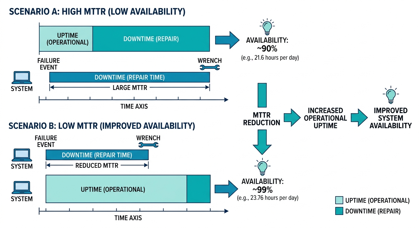
Increasing operational availability from \(98.81\%\) to \(99.70\%\) reduces total annual system downtime from \(103.9 \text{ hours}\) to \(26.2 \text{ hours}\), reclaiming \(77.7 \text{ hours}\) of operating capacity per year.
Implementing an Effective Asset Health Strategy
Transitioning from calendar-based maintenance to condition-based interventions requires a structured execution model:
- Perform Asset Criticality Ranking: Direct capital and sensor deployment to high-criticality equipment where unscheduled downtime causes severe safety risks or high financial losses.
- Select Target Modalities: Map failure modes identified in FMECA to matching diagnostic sensors (e.g., envelope acceleration for rolling element bearings, oil analysis for closed gearboxes, MCSA for submerged drives).
- Establish Baseline Trends: Set statistical alarm thresholds based on standard deviations from baseline operating data rather than relying solely on generic industry standards.
- Close the Maintenance Loop: Integrate diagnostic alerts into Computerized Maintenance Management Systems (CMMS) to trigger automated work orders when alert thresholds are breached.
To evaluate asset performance, calculate baseline reliability metrics, and model operational availability improvements, explore the interactive engineering tools available at ReliabilityCalc.com.