
A industrial plant carrying $1.5 million in slow-moving spare parts often experiences the same unplanned downtime as a facility with zero inventory. The root issue is not capital allocation—it is poor stocking strategy. Standard commercial retail inventory models assume continuous, predictable demand driven by purchasing cycles. When applied to maintenance, repair, and operations (MRO) materials, these models fail because component consumption is discrete, stochastic, and dictated by equipment failure physics.
Optimizing spare parts inventory requires integrating reliability engineering with statistical inventory control. Reorder policies must be grounded in failure distributions, supplier lead-time variance, and downtime consequences.
Criticality Stratification via the ABC-VED Matrix
Applying a single inventory policy across all SKUs leads to overstocking non-critical commodities while under-protecting single-point-of-failure assets. Financial metrics like annual dollar usage do not reflect operational risk: a $50 mechanical seal can trip an entire production line, while a $5,000 spare motor may serve a redundant unit.
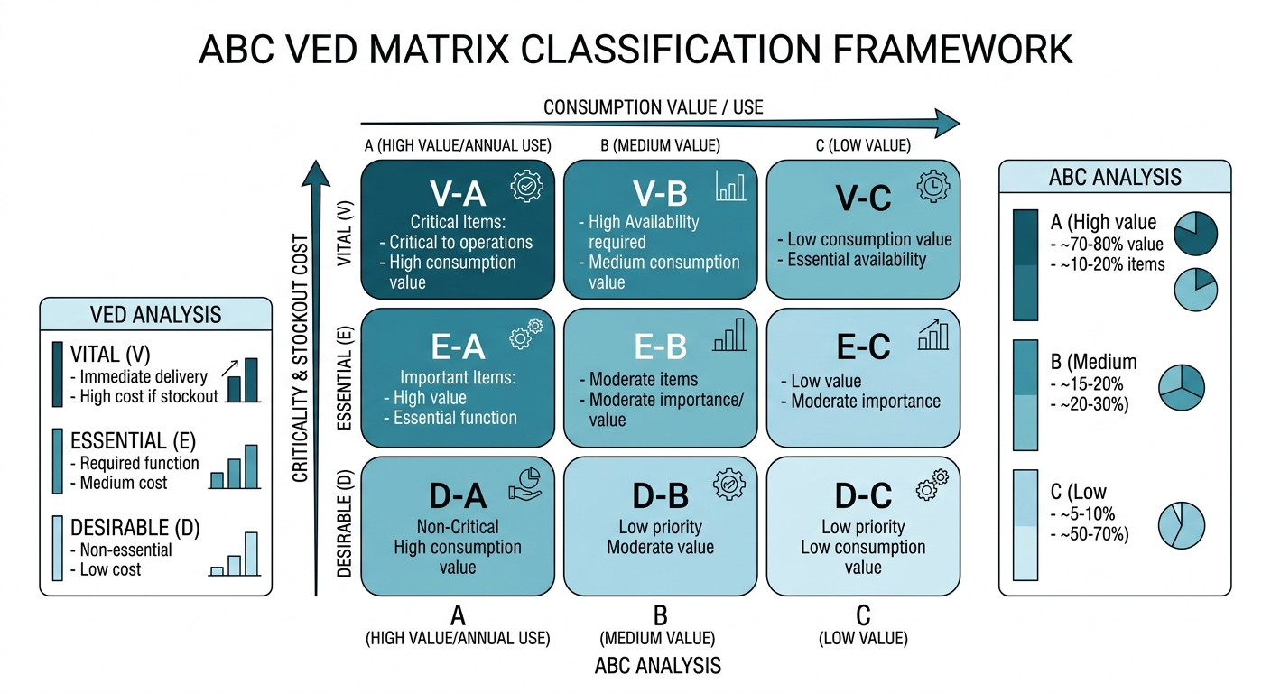
To establish a defensible stocking baseline, merge financial consumption value (ABC analysis) with operational criticality (VED analysis: Vital, Essential, Desirable):
- Vital (V): Failure triggers immediate safety risks, regulatory violations, or total plant outage with zero redundancy.
- Essential (E): Failure degrades capacity or causes partial system outage; limited short-term redundancy exists.
- Desirable (D): Failure has minimal impact on production; full redundancy exists or parts are available locally within acceptable lead times.
Integrating these dimensions creates a nine-cell matrix that determines stocking policies and control rigor. Spend profiles can be isolated using a Pareto Chart Tool to identify the high-value minority of SKUs requiring continuous review.
| Criticality Class | High Spend (Class A) | Medium Spend (Class B) | Low Spend (Class C) |
|---|---|---|---|
| Vital (V) | Continuous review (Min-Max); dual sourcing; consignment stock | Fixed Reorder Point (ROP); 1–2 unit safety buffer | Min-Max policy; high safety stock buffer carried |
| Essential (E) | Vendor-managed inventory (VMI); periodic review | Standard ROP based on lead-time variance | Two-bin Kanban; bulk replenishment |
| Desirable (D) | Order on demand; zero safety stock | Order on demand; standard supplier lead time | Reorder upon consumption; visual review |
Figure 1: ABC VED matrix classification framework
Mathematical Framework for Failure-Driven Reorder Points
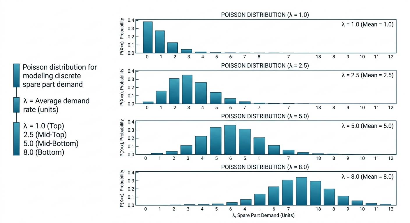
During the useful life phase of physical assets, component failures occur randomly at a constant mean rate (\(\lambda\)). Demand events follow a Poisson process. Baseline failure rates can be derived from operating logs or modeled with a Failure Rate Calculator.
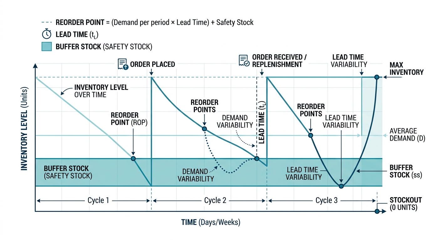
An optimal Reorder Point (\(ROP\)) accounts for expected lead-time demand while buffering against variance in both consumption rates and supplier fulfillment speed.
Expected demand during lead time (\(D_L\)) is:
$$D_L = d \cdot L$$
Where \(d\) is the mean demand per unit time and \(L\) is the mean supplier lead time in matching time units.
When demand and lead time are both variable, the required safety stock (\(SS\)) under continuous monitoring is calculated using the combined standard deviation (\(\sigma_{LT}\)):
$$\sigma_{LT} = \sqrt{L \cdot \sigma_d^2 + d^2 \cdot \sigma_L^2}$$
$$SS = Z \cdot \sigma_{LT}$$
Where:
- \(Z\) is the normal distribution factor for the target cycle service level (\(Z = 1.645\) for 95%, \(Z = 2.054\) for 98%, \(Z = 2.326\) for 99%).
- \(L\) is the mean procurement lead time.
- \(d\) is the mean periodic demand rate.
- \(\sigma_d\) is the standard deviation of periodic demand.
- \(\sigma_L\) is the standard deviation of lead time.
Combining expected lead-time demand and safety stock gives the final Reorder Point (\(ROP\)):
$$ROP = D_L + SS = (d \cdot L) + \left(Z \cdot \sqrt{L \cdot \sigma_d^2 + d^2 \cdot \sigma_L^2}\right)$$
Figure 2: Inventory reorder point buffer dynamics
Worked Numeric Example: Sizing Safety Stock for Critical Impellers
A chemical plant operates six identical centrifugal pumps continuously. Each pump uses a high-alloy impeller vulnerable to erosive wear. The engineering team must establish the \(ROP\) and \(SS\) for replacement impellers.
Input Parameters
- Operating assets (\(N\)): \(6\) units
- Operating hours per asset per year (\(H_a\)): \(8,000\) hours
- Total operational exposure (\(H_{total}\)): \(6 \cdot 8,000 = 48,000\) asset-hours/year
- Mean Time Between Failures (\(MTBF\)): \(6,000\) operating hours (validated via MTBF Calculator)
- Annual failure rate (\(\lambda\)): \(\frac{1}{6000} = 0.0001667\) failures/hour
- Annual expected demand (\(d_{annual}\)): \(48,000 \cdot 0.0001667 = 8.0\) impellers/year
- Monthly demand rate (\(d\)): \(\frac{8.0}{12} = 0.667\) impellers/month
- Standard deviation of monthly demand (\(\sigma_d\)): \(0.85\) impellers/month
- Mean procurement lead time (\(L\)): \(3.0\) months
- Standard deviation of lead time (\(\sigma_L\)): \(0.75\) months
- Target cycle service level: \(98\%\) (\(Z = 2.054\))
Step 1: Expected demand during lead time (\(D_L\))
$$D_L = d \cdot L = 0.667 \cdot 3.0 = 2.0 \text{ units}$$
Step 2: Combined standard deviation across lead time (\(\sigma_{LT}\))
$$\sigma_{LT} = \sqrt{L \cdot \sigma_d^2 + d^2 \cdot \sigma_L^2}$$
$$\sigma_{LT} = \sqrt{3.0 \cdot (0.85)^2 + (0.667)^2 \cdot (0.75)^2}$$
$$\sigma_{LT} = \sqrt{3.0 \cdot 0.7225 + 0.4444 \cdot 0.5625}$$
$$\sigma_{LT} = \sqrt{2.1675 + 0.2500} = \sqrt{2.4175} \approx 1.555 \text{ units}$$
Step 3: Required Safety Stock (\(SS\))
$$SS = Z \cdot \sigma_{LT} = 2.054 \cdot 1.555 = 3.194 \text{ units}$$
Since physical spares are discrete units, round up to preserve the targeted confidence level: \(SS = 4 \text{ units}\).
Step 4: Final Reorder Point (\(ROP\))
$$ROP = D_L + SS = 2.0 + 4 = 6 \text{ units}$$
Execution: Reorder when available inventory (on-hand + on-order - allocations) drops to \(6\) units. Holding \(4\) safety units buffers against demand surges and vendor lead-time delays.
Figure 3: Poisson probability distribution for spare part demand
Balancing Holding Costs Against Stockout Consequences
Targeting a blanket 99% service level across all inventory drives up carrying costs without delivering operational value. The optimal service level balances the annual holding cost of stock against the financial risk of unmitigated downtime.
Annual unit holding cost (\(H\)) is:
$$H = C_p \cdot i$$
Where \(C_p\) is unit purchase price and \(i\) is annual carrying cost percentage (typically 18%–25%, encompassing capital, warehousing, insurance, tax, and obsolescence).
The target economic fill rate (\(SL^*\)) is calculated using critical ratio optimization:
$$SL^* = \frac{C_s}{C_s + H}$$
Where \(C_s\) is the total stockout penalty (lost production margin, labor overtime, emergency freight, and expediting fees). Downtime losses can be quantified using a Downtime Cost Calculator.
Example Evaluation
A pump seal costs \(C_p = \$4,000\) with carrying rate \(i = 0.20\):
$$H = 4,000 \cdot 0.20 = \$800/\text{year}$$
If a stockout causes 6 hours of downtime at \(\$12,000/\text{hour}\), \(C_s = \$72,000\).
$$SL^* = \frac{72,000}{72,000 + 800} = \frac{72,000}{72,800} \approx 98.9\%$$
This justifies holding safety stock. Conversely, for a non-critical part where \(C_s = \$1,500\) and \(H = \$300\):
$$SL^* = \frac{1,500}{1,500 + 300} = \frac{1,500}{1,800} \approx 83.3\%$$
High safety buffers for non-critical parts are financially counterproductive.
Operational Execution Strategy
To maintain optimized stocking policies:
- Maintain Master Data Rigor: Standardize part nomenclature, verify OEM numbers, and link every SKU to specific Bill of Materials (BOM) assets. Disconnected catalog records cause duplicate stocking.
- Update Parameters Dynamically: Failure rates (\(\lambda\)) and lead times (\(L\)) drift over time. Recalibrate control parameters annually or after significant operating changes.
- Mitigate Slow-Mover Capital: For expensive capital spares (Class A-Vital), use vendor-managed inventory, regional pooling, or contractual lead-time guarantees to minimize direct ownership costs.
Spare parts optimization is a probabilistic engineering problem. Grounding inventory decisions in failure distribution parameters, lead-time dynamics, and cost consequences eliminates stockouts while freeing up working capital. Explore additional engineering utilities and reliability modeling tools at ReliabilityCalc.com.