
Accumulating unexecuted work orders in an industrial computerized maintenance management system (CMMS) is rarely just evidence of technician underperformance. Instead, it indicates a structural mismatch between work generation rates and net direct maintenance capacity. Left unmanaged, an unchecked work queue distorts weekly labor scheduling, masks emerging asset degradation, and pushes maintenance operations into reactive emergency response.
To maintain control over equipment reliability, maintenance engineering teams must treat the backlog not as a static task list, but as a dynamic control variable. Managing this balance requires clear queue taxonomy, precise mathematical labor modeling, quantitative risk-based prioritization, and routine backlog hygiene.
Taxonomy and Categorization of Work Queues
Lumping all uncompleted work orders into a single sum creates a misleading metric. A mature maintenance organization segregates work orders based on planning state and execution readiness. Proper classification prevents schedulers from releasing jobs that lack materials, permits, or operational access.
Maintenance work demand falls into four distinct operational categories:
- Ready-to-Work (Executable) Backlog: Fully planned tasks with all replacement parts staged, job safety analyses approved, line clearance secured, and labor estimated. This queue forms the direct input for weekly scheduling.
- Pending (Blocked) Backlog: Identified corrective tasks that cannot proceed immediately due to external constraints, such as engineering design reviews, long-lead procurement, contractor availability, or operational lockout dependencies.
- Outage/Turnaround Backlog: Validated corrective, preventive, or overhaul jobs that intentionally require a partial or total plant shutdown to execute safely.
- Unplanned (Draft) Queue: Newly submitted work requests awaiting field triage, planning, cost estimation, and material sourcing.
Figure 1: Classification of maintenance backlog components
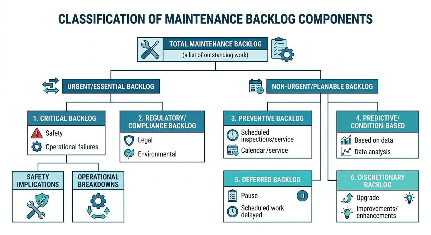
Tracking these categories independently ensures schedulers build weekly execution plans using only executable tasks, avoiding wasted craft hours spent searching for missing spare parts or waiting on clearances.
Quantifying Backlog in Crew-Weeks
Evaluating backlog by simple work order count or raw labor hours fails to account for craft specialization and real-time direct capacity. The standard metric for work volume is crew-weeks of backlog (\(B_w\)), defined as the time required for a dedicated craft group to clear all active approved work assuming no new work orders enter the queue.
Calculating crew-weeks requires adjusting gross labor hours down to net direct execution capacity to account for administrative duties, safety briefings, training, and leave.
Mathematical Model
Gross weekly craft capacity \(C_{\text{gross}}\) for a given craft is calculated as:
$$C_{\text{gross}} = N_{\text{tech}} \cdot H_{\text{shift}}$$
Where:
- \(N_{\text{tech}}\) = Number of active technicians in the craft group
- \(H_{\text{shift}}\) = Standard weekly shift hours worked per technician
Net direct labor execution capacity \(C_{\text{net}}\) accounts for indirect overhead and expected absenteeism:
$$C_{\text{net}} = C_{\text{gross}} \cdot (1 - P_{\text{indirect}}) \cdot \eta_{\text{avail}}$$
Where:
- \(P_{\text{indirect}}\) = Percentage of shift time spent on indirect tasks (meetings, toolbox talks, administrative logs)
- \(\eta_{\text{avail}}\) = Attendance availability factor adjusting for paid time off, sick leave, and training (\(0.0 \le \eta_{\text{avail}} \le 1.0\))
The backlog duration in crew-weeks \(B_w\) for a given volume of executable work \(H_{\text{ready}}\) is:
$$B_w = \frac{H_{\text{ready}}}{C_{\text{net}}}$$
Worked Numeric Example
A mechanical maintenance team supporting a processing unit needs to establish its current executable backlog duration.
Input Parameters:
- Active mechanical technicians (\(N_{\text{tech}}\)): \(8\text{ technicians}\)
- Standard shift schedule (\(H_{\text{shift}}\)): \(40\text{ hours/week per technician}\)
- Indirect labor overhead (\(P_{\text{indirect}}\)): \(12\%\text{ } (0.12)\)
- Craft availability factor (\(\eta_{\text{avail}}\)): \(85\%\text{ } (0.85)\)
- Approved executable work order hours (\(H_{\text{ready}}\)): \(952\text{ labor hours}\)
Step 1: Compute gross weekly labor capacity
$$C_{\text{gross}} = 8 \cdot 40 = 320\text{ labor hours/week}$$
Step 2: Compute net available direct execution capacity
$$C_{\text{net}} = 320 \cdot (1 - 0.12) \cdot 0.85$$
$$C_{\text{net}} = 320 \cdot 0.88 \cdot 0.85 = 239.36\text{ direct labor hours/week}$$
Step 3: Calculate crew-weeks of ready-to-work backlog
$$B_w = \frac{952}{239.36} \approx 3.98\text{ crew-weeks}$$
Interpretation:
The mechanical craft holds \(3.98\text{ crew-weeks}\) of executable work. If incoming demand consistently exceeds \(239.36\text{ hours/week}\), work queue depth will expand, increasing repair lead times. Craft execution efficiency and repair duration trends can be tracked alongside duration metrics using the MTTR Calculator.
Prioritization Frameworks for Work Queues
When work demand exceeds weekly craft capacity, maintenance organizations must use transparent, deterministic prioritization methods rather than relying on subjective user requests or first-in, first-out (FIFO) scheduling.
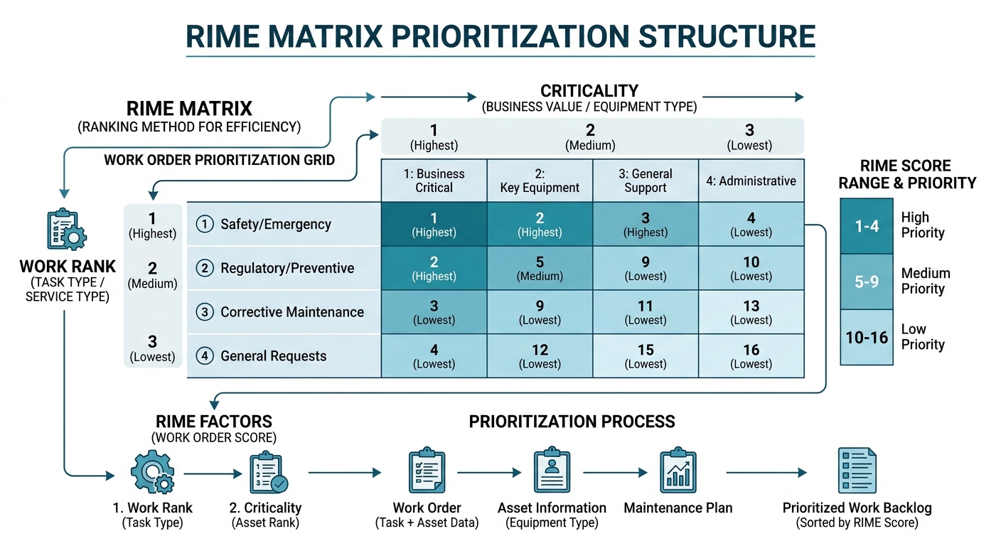
A quantitative method widely used in asset-intensive industries is the Ranking Index for Maintenance Expenditures (RIME), also called the Relative Importance Strategy Matrix. RIME establishes a priority score by multiplying an Asset Criticality Rating (\(A_c\)) by a Work Type Severity Score (\(W_s\)):
$$\text{RIME Score} = A_c \cdot W_s$$
Both scales typically range from 1 to 10, producing a priority index between 1 (lowest priority) and 100 (highest priority).
Figure 2: RIME matrix prioritization structure
The table below compares common prioritization frameworks used in industrial maintenance operations:
| Framework | Primary Basis | Key Strengths | Pitfalls & Limitations | Ideal Application |
|---|---|---|---|---|
| First-In, First-Out (FIFO) | Work submission timestamp | Simple; eliminates queue manipulation | Ignores asset criticality and risk; urgent repairs wait behind routine jobs | Facilities management with uniform, non-critical assets |
| Risk-Based Matrix | Consequence \(\times\) Likelihood of failure | Directly aligns with process safety, environmental, and regulatory standards | Subject to scoring variance between individual estimators | Capital-intensive process and chemical plants |
| RIME System | Asset Criticality \(\times\) Work Class | Objective, repeatable, transparent; mathematically structured | Requires an established, audited asset criticality ranking baseline | Medium-to-large multi-asset industrial facilities |
| Financial Risk / Cost Impact | Hourly production loss rate ($/hr) | Aligns maintenance scheduling directly with plant financial metrics | Difficult to quantify exact monetary risk for minor defect work orders | High-throughput continuous production lines |
When sorting queues using financial risk metrics, reliability managers can quantify the hourly downtime exposure of delayed jobs using the Downtime Cost Calculator. To identify key asset classes driving backlog growth, teams can apply the Pareto Chart Tool to isolate the vital few equipment types generating the majority of pending work orders.
Target Benchmarks and Burn-Down Strategies
Maintaining optimal queue depth requires balancing two operational risks: excessive backlog (causing delayed repairs and run-to-failure conditions) and insufficient backlog (causing craft idle time and low schedule compliance).
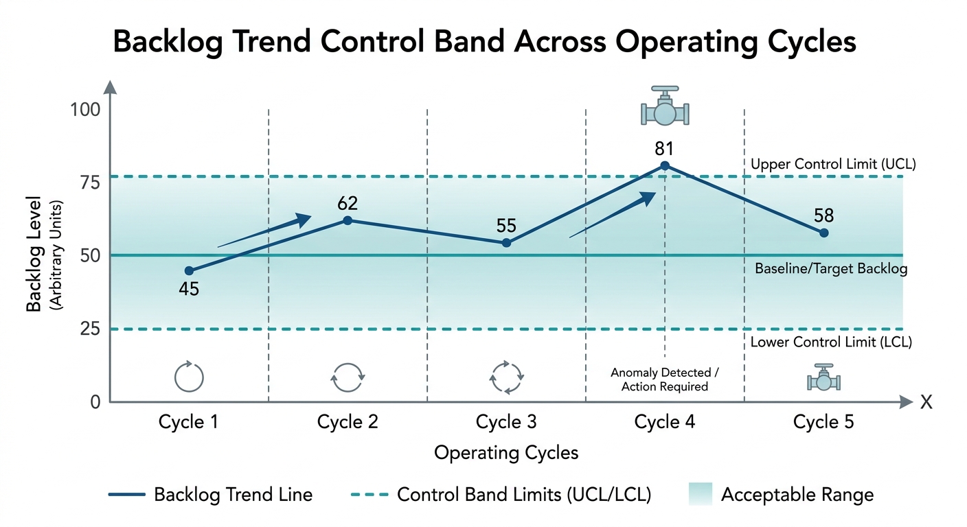
Recommended control bands for maintenance organizations are:
- Ready-to-Work Backlog: \(2.0 \text{ to } 4.0\text{ crew-weeks}\)
- Total Backlog (All Categories): \(4.0 \text{ to } 8.0\text{ crew-weeks}\)
Figure 3: Backlog trend control band across operating cycles
Managing Out-of-Control Backlogs
When executable backlog exceeds \(6.0\text{ crew-weeks}\), immediate corrective action is required to reduce equipment failure exposure. Operational strategies to burn down an inflated queue include:
- Backlog Audits and Scrubbing: Systematically cancel or consolidate obsolete work orders. Field audits in mature plants show that \(15\%\) to \(25\%\) of aging work orders often represent duplicate requests, self-corrected issues, or tasks rendered obsolete by modifications.
- PM Optimization: Temporarily adjust preventive maintenance frequencies. Suspend low-risk routine inspections if PM task volume is crowding out critical corrective actions.
- Capacity Augmentation: Deploy contractors for targeted, short-term backlog clearance campaigns without permanently increasing plant headcount.
- Scope Control Gatekeeping: Enforce strict gatekeeper reviews to prevent non-essential enhancements and convenience requests from entering the active CMMS queue.
Conversely, if executable backlog drops below \(1.0\text{ crew-week}\), craft crews face idle time, leading to lower execution productivity. Schedulers should pull forward non-urgent PMs or convert deferred maintenance tasks into active execution queues. Stabilizing this work balance directly supports long-term equipment uptime, which can be monitored using the Availability Calculator.
Conclusion
Managing maintenance queues effectively requires more than clearing work orders; it demands continuous capacity modeling, objective prioritization using frameworks like RIME, and disciplined queue maintenance. By keeping ready-to-work backlog within target limits of 2.0 to 4.0 crew-weeks, reliability teams protect asset health while maximizing labor productivity. To analyze your plant's operational performance metrics and model system risk, explore the calculation tools available at ReliabilityCalc.com.